Predicting Second-Hand Housing Prices in Beijing: A Comparative

Study of Machine Learning and Ensemble Models

Jia He

School of Information Engineering, China University of Geosciences (Beijing), Beijing, 100083, China

Keywords: Housing Price Prediction, Machine Learning, Ensemble Model, Web Crawler.

Abstract: In recent decades, the real estate market has always been an imperative force boosting China’s economic

development. Accurate housing price prediction plays a key role in policymaking and investment decisions.

Nonetheless, the traditional models often fall short when dealing with complex and nonlinear relationships.

This study focuses on predicting second-hand housing prices in Beijing using machine learning techniques.

The web crawler is used to obtain historical transaction data, then yield a dataset that includes 56,793 records

with 23 features after pre-processing in Beijing. Three models-Random Forest, XGBoost, and LightGBM-

were trained using grid-search and five-fold cross-validation. A combined ensemble model was also built to

improve the overall robustness. Evaluation and visualizations were used to compare performance. The

ensemble model outperformed the single model, followed by XGBoost, Random Forest, and LighGBM. This

paper aims to provide a new idea for house price prediction research through machine learning methods,

hoping to bring some inspiration to theoretical research and practical applications in related fields.

1 INTRODUCTION

In recent decades, the real estate industry has been a

vital engine driving economic growth in China

(Huang et al., 2021; Tang et al., 2016). Houses are not

only important fixed assets for people for either

residing or investing, but also the trading of houses

motivates plenty of related industries. Therefore,

accurate house price prediction plays a crucial role in

policy making, investment strategies, and urban

planning (Liu & Xiong, 2018). Nonetheless, due to

the multiple and non-linear factors influencing the

price--such as location, transportation convenience,

and interior decoration, the traditional linear

regression model cannot capture these features well

and give people a meaningful reference. At the same

time, with the rapid development and high reliability

of computational power (Thompson et al., 2020), this

study decides to utilize machine learning technology

to tackle these issues.

This study focuses on predicting second-hand

house prices in Beijing, the most energetic and

variable real estate market in China. To achieve this,

this study will construct advanced machine learning

models and optimize them for predictive work,

https://orcid.org/0009-0007-9926-2690

including Random Forest, XGBoost, and LightGBM.

Furthermore, considering each model cannot cover all

situations when prediction and there must be flaws in

some special facets, the paper will adopt an ensemble

strategy, weighted-averaging, to enhance the overall

behavior as a combined model. Eventually, the

combined model will offer significant insight into the

real estate market for homebuyers, real estate

investors, and government agencies for future plans.

The paper proceeds with the following

organization: Chapter 2 is Dataset obtained and pre-

processed, explaining how to obtain data via web

crawler, and data cleaning, feature generating, data

encoding, and normalization. Chapter 3 is Method,

presenting three models with their theories, including

Random Forest, XGBoost, LightGBM, and the

ensemble techniques. Chapter 4 is Experiment &

Analysis, elaborating details about the experimental

setup, and hyperparameter tuning by Grid Search

optimization. Chapter 5 is Results, displaying the

output of prediction. Chapter 6 is the Conclusion,

summarizing the whole study.

574

He, J.

Predicting Second-Hand Housing Prices in Beijing: A Comparative Study of Machine Learning and Ensemble Models.

DOI: 10.5220/0014363000004718

Paper published under CC license (CC BY-NC-ND 4.0)

In Proceedings of the 2nd International Conference on Engineering Management, Information Technology and Intelligence (EMITI 2025), pages 574-582

ISBN: 978-989-758-792-4

2 DATASET OBTAINED AND

PREPROCESSED

2.1 Dataset Obtained

In order to obtain reliable data, this paper chooses the

Lianjia website to access historical records. Lianjia is

one of the most influential real estate transaction

companies in China, and its website includes

tremendous data on houses.

Web crawler is a technique that can automatically

traverse web pages and extract target information. Its

basic process includes web requests, getting

responses, analysing content, extracting data, and

storage. In this study, the dataset comes from a web

crawler program in Python.

Here is the explanation of the web crawler’s

working:

Step 1, setting the target website’s URL list,

making the program request them in turn. Step 2,

sending a request to the website server with headers

that include details of the terminal that sends requests,

to decline the possibility of being recognized as a

crawler. Step 3, sometimes the website requires

passing a Captcha. By finishing it manually, the

program can work continuously. However, Captcha

will only show up several times at the beginning, and

will not interrupt the program later. Step 4, receiving

web source code. Decoding source code into HTML

using the function of the Beautiful Soup package in

Python. Step 5, Search and extract the needed

information from HTML. Step 6, storing information

in Excel. Step 7, getting the next URL in the list and

enter the next circulation. The following Figure 1

shows it directly:

Figure 1: Flowchart of Crawler Program Operation (Picture

credit: Original)

2.2 Data Basic Information

After crawling, the dataset has 73,952 data. There are

20 features in total displayed in Table 1:

Table 1: Features in Dataset

Feature Ex

lanation Exam

Region Administrative district Haidian

Business district Surrounding commercial area Jingsong

Communit

ecific residential communit

Jin

uan

Area Overall residential floor area

(

m²

)

132.0

Longitude Geographic coordinate measuring east-west position of a

communit

116.475053

Latitude Geographic coordinate measuring the north-south position

of a communit

39.885225

Layout Housing arrangement 4 bedrooms, 2 living room, 1 kitchen and 2

athrooms

Floor Number of floor levels

and label of it

High-floor (28 floor)

Orientation The main light-receiving surface of the housing North

Buildin

e T

e of construction Towe

Structure t

e Structural material Steel-concrete

Yea

The time when the building was finishe

2008

Decoration status Interior finishing condition of housing Hardcove

Heating method How the housing is

heated in winte

Centralized heating

Predicting Second-Hand Housing Prices in Beijing: A Comparative Study of Machine Learning and Ensemble Models

575

Feature Ex

lanation Exam

Elevato

Whether or not the building has at least one elevato

Yes or No

Transaction

ownershi

Legal form of housing transaction Commercial housing

Usage Designated function of housing Villas

Years of holding How long the current owne

has held the property More than 5 years

Ownership Nature of housing ownership rights Non-share

Price Total price of housing

(×10,000 RMB)

328.0

2.3 Data Cleaning

The obtained data needs to be cleaned. By filling in

the data features, discarding partial incomplete

records, and extracting the feature keywords,

enhancing dataset quality for later data pre-processed

and modelling.

The first step is filling in the data features.

Especially, there are keywords No data shown in two

columns-Year and Heating method. Considering that

in one community, the time when the building was

constructed and the Heating method are almost the

same. For these data, searching for other data whose

Community is the same. Then, firstly take the average

number of their Year column, then replace No data

with the number in the Year column. Secondly, taking

the majority type in the Heating method column, then

replacing No data with the type in the Heating method

column.

The second step is deleting features. Given that

Community has 5809 categories and each category

has approximately 5 data only after pre-processing,

this paper decides to delete this feature because

Community will hardly offer a contribution to price

prediction. Moreover, it is not meaning to analyse

Latitude and Longitude in numerical form, so this

study deletes these two features as well.

The third step is discarding data with missing

values. The proportion of data with missing values is

relatively low like 1.03% and 0.23% in the specific

columns, so this study decides to discard these data.

Eventually, the remaining dataset has 56793

pieces of data, which is enough for training and

testing models.

2.4 Generating Features

To improve models’ behaviors significantly, this

study generated 2 key features by utilizing the

features Longitude and Latitude.

City ring zone: Refers to the housing location

based on Beijing’s ring road(e.g., 2nd Ring, 3rd

Ring). By setting points and connecting them to

outline each area on Google map, this study obtains

each point’s latitude and longitude precisely.

Therefore, we can judge each housing with their

locations belonging to which city ring zone. The

closer to the city center (inner rings), the more central

and expensive the area tends to be.

Subway: How far is the housing from the nearest

subway station. The closer to the subway station, the

more expensive the housing is relative. To obtain

each station’s location, this study wrote Overpass

Query Language and ran it on the Overpass Turbo

website, searching for all subway stations in the area

of Beijing and their latitude and longitude

coordinates, and exporting and processing them as

csv files.

Each housing’s location is compared to a dataset

including all subway stations over the coordinate of

latitude and longitude, this study uses the Geodesic

distance algorithm to transform longitude and latitude

between two points into straight-line

distance(meters), which is based on the WGS-84

ellipsoid.

For the column Layout, there are actually 4

features and this study decides to split them into 4

new features bedroom_Layout, living_room_Layout,

kitchen_Layout, bathroom_Layout. For example, 4

bedrooms, 2 living rooms, 1 kitchen and 2 bathrooms

will be separated into 4 columns, reducing the

dimensions of the dataset and increasing the

interpretability of the models.

2.5 Encoding

Map coding is a popular way to transform text into a

number, facilitating building models later. This study

adopts this way to encode every column, whose

values are text.

Business district, Construction type, and

Decoration status are encoded using the sequential

encoding method(Zaraket et al., 2006). The

remaining features are encoded by manual mapping.

There are 16 features required to be encoded.

After encoding, all the values have been numbered

now.

EMITI 2025 - International Conference on Engineering Management, Information Technology and Intelligence

576

2.6 Normalization

In this study, Z-score normalization was employed to

standardize feature values across various scales. The

normalization formula is:

𝑧=

𝑥−μ





Where 𝑥 indicates the raw data point, μ

corresponds to the mean of the dataset, and σ refers

to the standard deviation. Eventually, the data of each

feature will be normalized to zero mean and unit

variance.

This method eliminates the negative effect of the

scale differences among variables, ensuring

comparability among variables.

3 METHOD

3.1 Random Forest

Random Forest serves as a powerful ensemble

method, which was originally introduced by Breiman

(Breiman, 2001). The reason this study chose

Random Forest is that, unlike parametric models,

Random Forest is particularly effective in handling

noisy data in high dimensions(Liaw & Wiener, 2002),

keeping flexibility and reducing variance when

predicting.

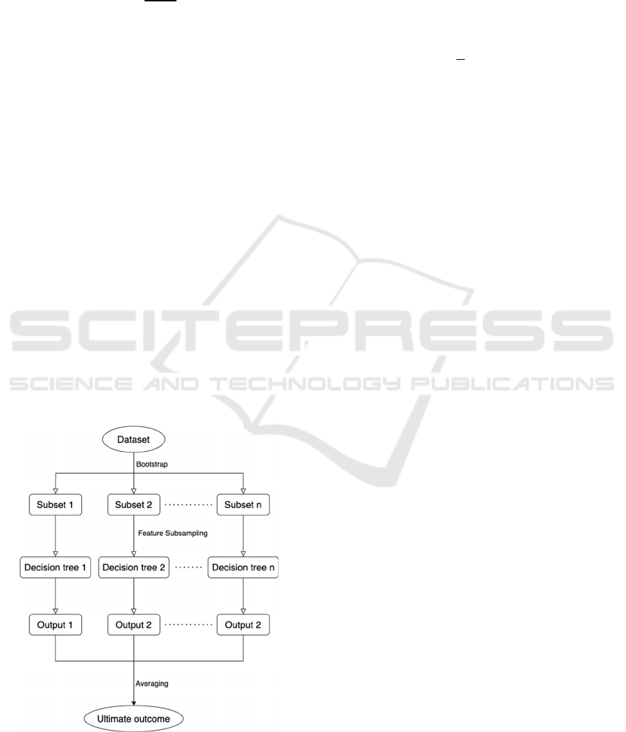
Figure 2 displays a basic schematic of how the

Random Forest works:

Figure 2: Flowchart of Random Forest (Picture credit:

Original)

Each regression decision tree is trained using a

bootstrap sample of the original data, and at each

node, a random subset of features is selected to

determine the best split, which decorates the trees and

enhances generalization performance(Biau, 2012).

Random Forest derives continuous output through

the aggregation of predictions by an array of decision

trees:

𝑦=

𝑇

ℎ





𝑥











Where T is the total tree count, with ℎ





𝑥



being

the prediction result from the t-th tree.

3.2 XGBoost

Extreme Gradient Boosting (XGBoost) is a type of

learning algorithm, recognized for its speed,

accuracy, and avoidance of overfitting over

regression tasks. Additionally, it is widely recognized

for handling structured data(Chen & Guestrin, 2016),

which is appropriate for the dataset in this study.

Unlike the method of building a decision tree in

Random Forest, XGBoost adopts a sequential

approach. The purpose of every subsequent tree is to

capture the residuals left by the prior prediction

round, which is the part that cannot be explained

former. As the number of trees, XGBoost will

gradually remedy the residuals, making the result

more precise.

The model output 𝑦



 is the sum of K regression

trees applied to input 𝑥



𝑦



=𝑓





𝑥









,𝑓



∈ℱ





Each tree 𝑓



comes from a function space of

decision trees ℱ. Moreover, XGBoost minimizes the

objective function containing the loss term and the

regularization term to prevent model overfitting:

ℒ=l













Ω













Where ℒ is the overall objective function,

𝑙



𝑦



,𝑦







is the loss between the true value 𝑦



and

predicted value 𝑦



, and Ω



𝑓





is the regularization

term that penalizes the complexity of tree 𝑓



3.3 LightGBM

A Light Gradient Boosting Machine (LightGBM) is a

kind of high-efficiency framework based on decision

Predicting Second-Hand Housing Prices in Beijing: A Comparative Study of Machine Learning and Ensemble Models

577

trees. LightGBM utilizes histogram-based split

finding, specializing in large-scale and high-

dimensional data(Ke et al., 2017). It is widely applied

in financial modeling and environmental forecasting

for regression problems(Wasserbacher & Spindler,

2022).

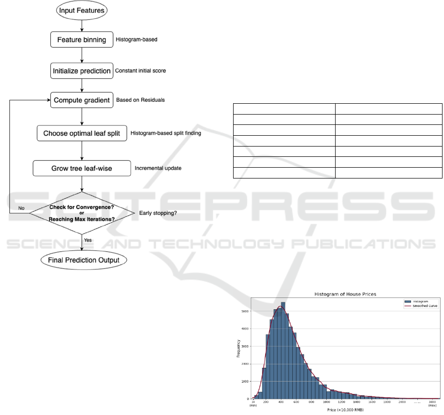
Following is a simple flowchart of the LightGBM,

shown in Figure 3:

Figure 3: Flowchart of LightGBM (Picture credit:

Original).

As the flowchart illustrates, LightGBM begins

with feature binning and initial prediction, followed

by computing gradients and selecting optimal splits.

It grows the leaf with the highest loss, allowing the

model to build deeper trees that reduce errors.

Furthermore, the model checks whether convergence

has been achieved. If not, it loops back to recompute

gradients for the next round of training.

3.4 Ensemble Method

This study uses weighted-average method to

ensemble three models.

This method in ensemble learning combines

multiple outputs by assigning each a weight based on

its performance. In this way, the final output can

generate or retain the best result from various angles

of analysis, and decrease the impact of weaker

models.

Using a numerical strategy, this study minimized

RMSE on the validation set to automatically adjust

the weight.

4 EXPERIMENT & ANALYSIS

4.1 Experimental Environment

The environment of this study includes a dataset, a

laptop. All experiments were implemented using

Pycharm and executed locally. Here is the

information in Table 2 of the laptop:

Table 2

Experiment Environment.

Item Details

Com

ute

MacBook Ai

Chi

le M2

Memory 8GB

Storage 512GB

Operating System Sonoma 14.4

IDE P

Charm 2024.1.6

4.2 Data Exploration

This study depicts the Histogram of House Prices,

House Price Distribution by Region, and Feature

Correlation Heatmap for a better understanding of the

dataset

4.2.1 Histogram of House Prices

Figure 4: Histogram of House Prices (Picture credit:

Original).

Figure 4 presents the house price distribution,

measured in units of ten thousand RMB. The majority

of houses are located between 200 and 800, with a

prominent peak at around 400, showing a clear right-

EMITI 2025 - International Conference on Engineering Management, Information Technology and Intelligence

578

skewed pattern. A fitted smoothed line emphasizes

the decline in frequency as prices increase.

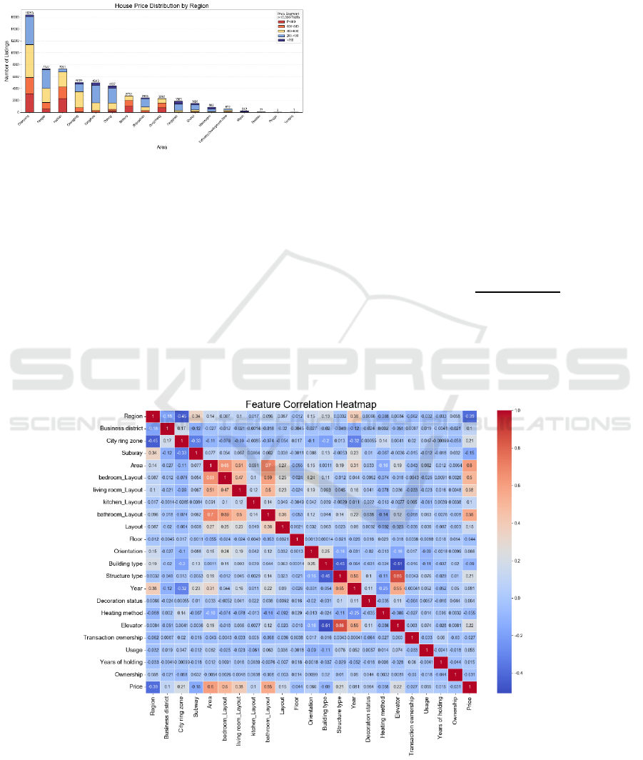
4.2.2 House Price Distribution by Region

Figure 5 House Price Distribution Chart (Picture credit:

Original).

Figure 5, a stacked histogram, vividly illustrates

the distribution of houses across five price ranges

within each region, with regions ranked from highest

to lowest in total transactions.

Chaoyang records the highest number of

transactions, with a relatively even distribution across

all price ranges except the lowest. Moreover, in

Haidian, Dongcheng, and Xicheng regions, high-

priced houses dominate, reflecting their central

location and well-developed infrastructure.

4.2.3 Feature Correlation Heatmap

Though Figure 6, is a correlation heatmap, it is clear

to see the correlation coefficient between any two

features. The price has a relatively high coefficient

with Area, Layout, and Region, indicating these

features influence price most.

5 EXPERIMENT & ANALYSIS

5.1 Experimental Environment

In order to compare each model’s performance, this

study adopts uniformly three indicators, 𝑅



， MAPE

and RMSE, to evaluate.

Coefficient of determination (𝑅



) assesses the

degree to which the variation in the target is explained

by the model. A value closer to 1 indicates better

predictive performance. Formula:

𝑅



=1−

∑

𝑦



−𝑦













∑

𝑦



−𝑦













where 𝑦



 is the predicted value, 𝑦



is the mean of

actual values, and 𝑛 is the number of samples. All of

them represent the same meaning in the formula

down below.

Figure 6: Feature Correlation Heatmap (Picture credit: Original).

Predicting Second-Hand Housing Prices in Beijing: A Comparative Study of Machine Learning and Ensemble Models

579

Mean Absolute Percentage Error(MAPE)

reflects the mean proportionate difference between

forecasts and true values. It indicates how accurate

predictions are in relative terms—a lower MAPE

means higher accuracy. Formula:

𝑀𝐴𝑃𝐸=

𝑛



𝑦



−𝑦





𝑦









×100%





Root Mean Squared Error(RMSE), as a

standard metric in regression analysis, evaluates

model accuracy by measuring the square root of the

mean squared discrepancy between predicted and

actual values. RMSE reflects the extent of the error

between the true value and the predicted value in

numerical form. Formula:

𝑅𝑀𝑆𝐸=



𝑛





𝑦



−𝑦

















5.2 Histogram of House Prices

For each model, this study uses the Grid Search

optimized algorithm to find the best combination of

parameters (Claesen & De Moor, 2015). Later,

utilizing 5-Fold Cross Validation to evaluate fairly

the hyperparameter combinations to identify the

model that generalized best to unseen data (Soper,

2021). Table 3, Table 4, Table 5 are the

hyperparameters of three models.

Table 3: Hyperparameters of Random Forest.

Hyperparameter Value Explanation

n_estimators 200 Numbe

of decision trees

max

th 10 Maximum de

th of each tree

min

sam

les

lit 2 Minimum sam

les to s

lit node

min

sam

les

leaf 1 Minimum sam

les in leaf node

Table 4: Hyperparameters of XGBoost.

Hyperparameter Value Explanation

n_estimators 400

umber of boosting rounds

max

th 9 Maximum tree de

learnin

rate 0.2 Ste

size shrinka

subsam

le 0.9 Row sam

lin

ratio

colsample_bytree 1 Column sampling per tree

Table 5: Hyperparameters of LightGBM.

Hyperparameter Value Explanation

n_estimators 150 Number of trees

max_depth -1 No tree depth limit

learnin

rate 0.1 Trainin

ste

size

num

leaves 70 Max leaves

er tree

Shown as three tables above, the key

hyperparameters and values of Random Forest,

XGBoost and LightGBM are different respectively.

6 RESULTS

6.1 Evaluating by Indicators

Table 6: Evaluation Results by Indicators.

Model

𝑹

𝟐

MAPERMSE Execution Time(s)

Random Forest 0.9205 8.62% 95.92 175.18

XGBoost 0.9254 7.66% 92.90 850.21

htGBM 0.9211 9.74% 95.58 42.46

Ensemble model0.9317 7.54% 88.88 1072.24

The evaluation is shown in Table 6. In single

model performance:

The 𝑅



of XGBoost is the minimum, suggesting

it has the best interpretation for the trend of housing

price fluctuations

The MAPE and RMSE of XGBoost are the

smallest in the single model’s performance,

suggesting it gives the best prediction of housing

price.

The execution time of LightGBM is the least

when losing little performance, suggesting it is the

most appropriate for the quick prediction of numerous

cases.

As expected, the ensemble model performs best in

all cases. Notably, 𝑅



and RMSE improves a lot,

though the execution time is the longest.

6.2 Evaluating by Visualizing

Since there are over 10 thousand data points in the

testing set, plotting all of them would make the charts

too dazzling to see clearly. Therefore, this study

divides these data into 100 groups and takes their

average price to compare to the predicted price:

EMITI 2025 - International Conference on Engineering Management, Information Technology and Intelligence

580

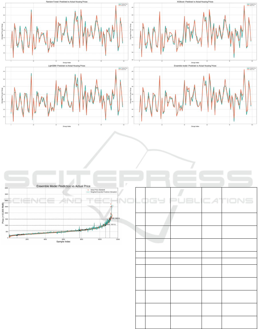
Figure 7: Evaluation Results by Visualizing (Picture credit: Original)

Figure 7 is a line chart between actual and

predicted housing prices showing the performance of

three models and the ensemble model directly. As the

charts illustrate, the effects, from best to worst, are:

Ensemble model, XGBoost, Random Forest and

LightGBM.

Figure 8 Ensemble Model Prediction (Picture credit:

Original)

Here is the final result, Figure 8, with all samples

in the testing set measured in units of ten thousand

RMB. This chart shows that in the price range

between 200 and 600, the prediction is fairly accurate.

In the range of 600-1500, the prediction presents little

fluctuations. And under 200 and beyond 1500, the

prediction can only catch the basic trend due to fewer

samples in this range.

The deviation of RMSE is mainly caused by high-

priced housing with prices above 600.

6.3 Examples

The following Table 7 shows details about

predictions on the testing set:

Table 7.

Actual

Price

(×10,000

RMB)

Predicted

Price

(×10,000 RMB)

Absolute

Error

Percentage

Error

352

280.0 281.968126 1.968126 0.70%

784

580.0 514.600970

65.39903

11.27%

997

335.0 330.706546 4.293454 1.28%

4 218.0 224.593320 6.593320 3.02%

…… … … …

589

1080.0 1032.699834

47.30016

4.37%

214

163.5 203.736533

40.23653

24.60%

115

1700.0 1538.769007

161.2309

9.48%

893

800.0 822.051541

22.05154

2.756443%

381

485.0 482.632405 2.367595 0.48%

Table 7 above shows there are discrepancies

between actual and predicted prices, with varying

error rates.

Predicting Second-Hand Housing Prices in Beijing: A Comparative Study of Machine Learning and Ensemble Models

581

7 CONCLUSION

This study utilizes web crawler technology to obtain

a dataset for historical transactions in Beijing. After

the data is pre-processed, there are 56793 pieces of

data with 23 features. With grid-search and 5-Fold

Cross Validation, training Random Forest, XGBoost,

LightGBM and the ensemble model to offer

predictions for housing price. Afterward, this study

evaluates each model by indicators and visualization.

The effects, from best to worst, are: Ensemble

model, XGBoost, Random Forest and LightGBM. As

the research results show, the ensemble method can

outperform a single model in complex real estate

prediction tasks. This study offers a comparison of

various models and emphasizes the strengths of

ensemble approaches.

This study offers a practical machine learning

method for real estate market prediction. It offers

meaningful insight for real estate analysts and

policymakers. Moreover, it contributes to the

growing body of research applying ensemble

methods to China’s housing prices.

Though the results are great, this study has the

limitation that the omission of inflation effects in the

time span of the dataset may constrain the model’s

interpretation to capture real-estate market trends

years later. Future studies can explore deeper time-

series models like ARIMA and introduce them into

an ensemble model, promoting long-term stability in

model outcomes.

REFERENCES

Biau, G. 2012. Analysis of a random forests model. Journal

of Machine Learning Research, 13, 1063–1095.

Breiman, L. 2001. Random forests. Machine Learning,

45(1), 5–32.

Chen, T., & Guestrin, C. 2016. XGBoost: A scalable tree

boosting system. In Proceedings of the 22nd ACM

SIGKDD International Conference on Knowledge

Discovery and Data Mining (pp. 785–794).

Claesen, M., & De Moor, B. 2015. Hyperparameter search

in machine learning. arXiv.

Huang, Y., Khan, J., Girardin, E., & Shad, U. 2021. The

role of the real estate sector in the structural dynamics

of the Chinese economy: An input–output analysis.

China & World Economy, 29(1), 61–86.

Ke, G., Meng, Q., Finley, T., Wang, T., Chen, W., Ma, W.,

... & Liu, T.-Y. 2017. LightGBM: A highly efficient

gradient boosting decision tree. In Advances in Neural

Information Processing Systems, 30 (pp. 3146–3154).

Liaw, A., & Wiener, M. 2002. Classification and regression

by randomForest. R News, 2(3), 18–22.

Liu, C., & Xiong, W. 2018. China’s real estate market

(NBER Working Paper No. 25297). National Bureau of

Economic Research.

Soper, D. S. 2021. Greed is good: Rapid hyperparameter

optimization and model selection using greedy k-fold

cross validation. Electronics, 10(16), 1973.

Tang, B., Liu, C., & Li, J. 2016. An investigation into real

estate investment and economic growth in China: A

dynamic panel data approach. Sustainability, 8(1), 66.

Thompson, N. C., Greenewald, K., Lee, K., & Manso, G. F.

2020. The computational limits of deep learning. arXiv.

Wasserbacher, H., & Spindler, M. 2022. Machine learning

for financial forecasting, planning and analysis: Recent

developments and pitfalls. Digital Finance, 4, 63–88.

Zaraket, F., Aziz, A., & Khurshid, S. 2006. Sequential

encoding for relational analysis. In Proceedings of the

18th International Conference on Computer Aided

Verification (CAV) (pp. 164–178). Springer.

EMITI 2025 - International Conference on Engineering Management, Information Technology and Intelligence

582