Research on the Factors Contributing to Change in Housing Price in

California

Ziyu Li

Social Sciences College, University of California, Irvine, Irvine, 92697, U.S.A.

Keywords: Housing Value, Correlation Coefficient, Linear Regression Model.

Abstract: Housing price is always the popular topic in the current market. To predict the alternation in housing price, it

is necessary to initially forecast the trend of those influencing factors. This article aims to investigate the

potential factors that influence alternation in housing prices. 20,640 samples from a dataset of California’s

housing group by 1990 will be conducted in this essay to complete further analysis. Then, this research will

measure correlation coefficients and employ linear regression model based on the eight variables shown from

the dataset. By searching for coefficient, unstandardized beta and variance inflation factor (VIF) value, this

research can conclude the most significant causes to affect housing prices. Finally, the research indicates that

income level is the main feature, other causes including housing ages, location as well as population can also

affect prices in some aspects. The data and purpose outcomes can provide households and housing agencies

direction regarding the trend of housing market.

1 INTRODUCTION

Housing price is one of the most pivotal indicators in

today’s society, affecting the entire economy and

people life. As housing acting as one of the

fundamental properties for people to require

maintaining normal life, it is the criteria to measure

people’s well-being and individual health, which

means lots to human beings (Rolfe et al, 2020). Due

to the extensive demand for shelters, property values

are now a controversial topic among academics and

the public. The importance of researching house

prices is further emphasized by the fact that real estate

is frequently seen as a worthwhile financial asset.

Housing prices in the United States have increased

rapidly and even dramatically over the last few

decades. Nowadays, house prices have become one of

the economies that employed adults care about the

most. Its price trend determines when people will

choose to buy or sell houses. Between 2020 and 2023,

California recorded its first population decline since

becoming a state in 1850 (Batdorf, 2024). This

unprecedented demographic change because of

multiple causes including high living expenses,

increasing remote work flexibility, family

considerations and potential economic challenges.

These shifts have highlighted the complex

relationship between changing population trends and

housing affordability in the state.

While, forecasting the price trends and

comprehending their wider economic impact require

a grasp of the elements that affect house values. This

study will examine and conclude home prices

according to existing housing data from California.

Besides, this research will also analyse the factors

influencing change in housing prices.

The housing price is definitely determined by

multiple features that surrounding housing itself,

housing locations and the entire society. From the

past, the theme has attracted by several researchers to

explore into. Those existing research offers extensive

theoretical models and empirical evidence examining

the key factors influencing housing prices. In the

research by Li and Yang, they employed a multiple

linear programming tool to analyse the key features.

By examining the linear relationship between a

dependent variable and multiple independent

variables, the model estimates regression

coefficients, and minimizes the difference between

the actual observed values and the values predicted by

the model. By comparison of different variable

combinations, the study aimed to identify the optimal

model for accurate housing prices forecasting (Li and

Yang, 2024).

468

Li, Z.

Research on the Factors Contributing to Change in Housing Price in California.

DOI: 10.5220/0014361300004718

Paper published under CC license (CC BY-NC-ND 4.0)

In Proceedings of the 2nd International Conference on Engineering Management, Information Technology and Intelligence (EMITI 2025), pages 468-473

ISBN: 978-989-758-792-4

Mao and Yao conducted a similar study using

the King County House Sales dataset to investigate

how geographic features impact housing price. In the

research, they apply multiple linear regression

(MLR) combined with 10-fold cross-validation to

assess model performance. The findings highlight

that factors including the number of bedrooms,

latitude, and longitude significantly affect. Their

predictive summary is both methodologically sound

and interpretable, offering detailed views into the

relationship between these variables and property

values (Mao and Yao, 2020). Additionally, Lau

analysed how population alternation and

homeownership rates impact California housing

prices from 2020-2022 potentially using county-level

data. This study applied time-series analysis and

correlation theory to measure relationships between

these variables, with results indicating positive,

negative, or neutral associations (Lau, 2024).

Yu applied the same linear regression analysis, the

common statistic method in order to predict the target

variable by linear combination of characteristic

variables. Evaluation of these models through

different matrixes such as mean square error is the

strategy she used to determine the accuracy of model,

which is indeed understandable and precise (Yu,

2024). Similarly, Yan also conducted excel to build

up a multi-regression model, aiming to research on

influencing factors of housing value in New York in

a comprehensive aspect (Yan, 2022). There are some

other researchers adopt different strategies to figure

out those potential causes. Zoppi et al. attempted to

employ Hedonic models to analyze environmental

and structural features which affects housing market

in Cagliari (Zoppi et al, 2015). Huang et al. conducted

models to study and collect those data of unusual

variation in housing prices (Huang et al., 2010). In

summary, this study will properly conduct the

combination of two strategies, correlation module and

linear regression, in order to investigate the potential

features that influencing change in housing prices in

California.

2 METHODS

2.1 Data Source

In this research, a dataset focuses on housing price

from Kaggle website will be adopted. This dataset

offers a practical starting point for exploring machine

learning techniques. It covers housing information

from the 1990 California census, measuring various

homes across different districts. This dataset includes

region-level statistics such as population, median

income and housing characteristics, providing an

understandable and clear background for building and

evaluating machine learning models. From the

original dataset, there were several missing values in

the total_bedrooms column. To deal with this issue,

the missing entries were occupied using the median

value. From the full set inputs, a random sample of

20640 records was selected for this research. Then,

the updated dataset now includes nine features-

longitude, latitude, housing median age, total rooms,

total bedrooms, population, households, median

income and ocean proximity, along with the target

variable, median house value.

2.2 Variables Explanation

In order to present the further model, the study needs

to initially list out all the dependent variables and the

independent variable that investigating in the dataset.

These variables cover longitude, latitude, housing

age, total rooms, total bedrooms, population,

households, income level, and the house value.

Therefore, the research lists out a relevant variables

table, as shown in Table 1.

Table 1: Variables introduction

Variables Description

Lon

itude House distance to the west

Latitude House distance to the north

Housin

e Median a

e of a house

Total Rooms Total room numbe

Total Bedrooms Total bedroom numbe

Population Total number of residents living

in a house

Households Total household numbe

Income Income level for households

House Value Median House

rice

2.3 Method Introduction

In this analysis, both correlation and linear regression

methods are used to investigate the potential factors

influencing housing prices in California. The initial

step is data cleaning, referring to handling missing

values, such as replacing null numbers in total

bedrooms with the median calculation as well as

dropping irrelevant columns like ocean proximity,

since it doesn’t change throughout the whole dataset.

Research on the Factors Contributing to Change in Housing Price in California

469

The correlation between median house value and

variables including longitude, latitude, housing

median age, total rooms, total bedrooms, population,

households, and median income is calculated, helping

determine which variables have relatively stronger

relationships with the house price.

After identifying those relevant variables through

correlation approach, this paper builds a multiple

linear regression model based on these indicators.

This model not only quantifies the influence of each

variable but also eliminate errors, for example two

variables are highly correlated, which may distort the

model accuracy. This research uses statistical tests

including p-values and R² scores in order to evaluate

the significance and explanatory power of the model.

In this study, the combination of correlation and

regression model provides a clearer understanding of

how those different features relate to housing prices

in California.

3 RESULTS AND DISCUSSION

3.1 Correlation Analysis

To investigate the relationship between housing value

and those potential influencing factors, this paper

attempts to conduct Pearson correlation analysis,

referring to a calculation measuring linear

relationship between two continuous variables. The

correlation coefficient is a result of ratio between

the covariance of two variables and the product of

their standard deviations (Asuero et al., 2007). Those

coefficients always are ranging from -1 to 1, a

positive value represents a direct relationship while a

negative value implies an inverse relationship.

After the implement of regression correlation

model, the standard deviation and mean of each

variable are figured out. Plugging those data into the

formula mentioned before, then this paper obtains the

correlation coefficient between each pair of two

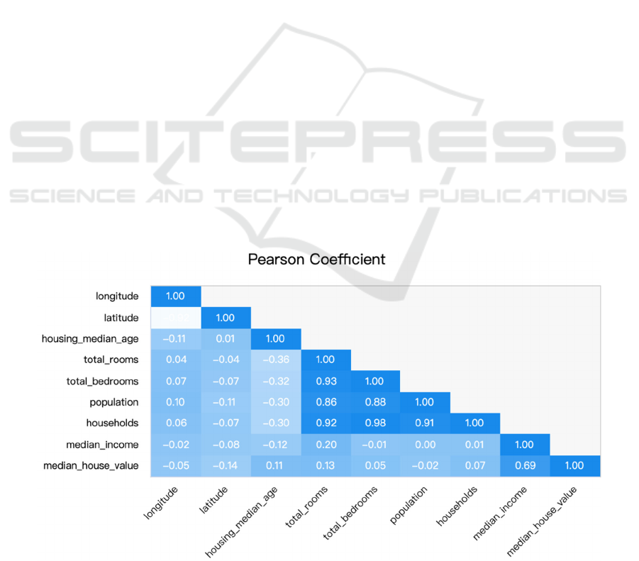
variables among those listed elements. Figure 1

shows the all the combinations; it indicates the

indexes of linear relationship between those factors

directly. From the figure 1, it is intuitive to determine

which pairs of variables maintain a strong correlation.

The diagram presents a strong relationship

between households and total bedrooms (0.98), total

rooms and total bedrooms (0.93), as well as total

rooms and population (0.92). These suggest that

families with more households require greater

amount of rooms and bedrooms, which is obvious.

Although using all the combination is direct to see

each variable, this study should focus more on the

factors influencing the housing value. Therefore, this

paper wipes off the other variables being target

variables in order to receive an updated correlation

diagram.

Figure 1: Pearson Coefficient Table for Variables (Picture credit: Original).

EMITI 2025 - International Conference on Engineering Management, Information Technology and Intelligence

470

Figure 2: Pearson Coefficient Table for Median Housing Value (Picture credit: Original).

From Figure 2, it is much more direct to witness the

potential causes to affect change in housing value.

Looking at the chart, the strongest relationship is

between income and house value. The correlation

coefficient between median_income and

median_house_value reaches to 0.69, which is a

relatively strong positive figure. That is probably

because households with higher income will prefer

houses in a higher price to satisfy their requirement of

higher living standard. Besides, wealthy people

always pursue shelters with superb location and

greater size, these factors will also impact a higher

housing price. Therefore, it’s reasonable that income

level is the most strongly and positively linked factor

to housing value.

Other factors like the number of rooms in a house

(total_rooms) and the age of the house

(housing_median_age) maintain weaker positive

relationships with housing prices. Sometimes housing

age cannot be a determination of housing prices as

new houses built in current years can be sold in a high

price because of its brand-new infrastructure and

novel layout. Consumers are likely to be attracted by

those factors, thus larger consumer groups increase its

demand, causing increase in price. However, aged

homes can also be set in a high price. Those homes

are often found in well-established neighborhoods

and hold a larger land size because land was cheaper

and more accessible at that time. Therefore, these

historical houses may also be popular among

consumers. Housing value, as well as can be properly

impacted by the room amounts, while it is reasonable

that room sizes should take into account when it

comes to the number.

Some variables including total bedrooms,

population as well as the households don’t seem to

affect house prices significantly, they maintain

correlation coefficients very close to zero. This

suggests that numbers of households and bedrooms

cannot be the determinations that influencing housing

value.

Finally, location, especially latitude, seems to

matter relatively. Latitude and longitude have small

negative correlations with house prices. This may

indicate that those houses located relatively inland or

farther north in California tend to become slightly

cheaper. As those homes are located far away from

main cities or the coast, the transportation could be

more inconvenient and time-consuming, therefore

demand on those houses will reduce, causing decline

in housing prices of homes.

3.2 Linear Model Results

After calculation of correlation coefficients, the linear

regression model should be conducted for the further

analysis and conclusion. This is a model that

estimates the relationship between dependent

variables and independent variables. As seen from

table 2, those eight dependent variables for linear

regression have established a model combined with

value of beta of each variable to calculate the housing

value.

Research on the Factors Contributing to Change in Housing Price in California

471

Table 2: Linear Regression Table

BSt

. E

Beta t P value VIF Tolerance

Constant -3585395.747 62900.543 - -57.001 0.000 - -

Longitude -42730.120 717.087 -0.742 -59.588 0.000 8.714 0.115

Latitude -42509.737 676.952 -0.787 -62.796 0.000 8.829 0.113

Housing median

1157.900 43.389 0.126 26.687 0.000 1.260 0.794

Rooms numbe

-8.250 0.794 -0.156 -10.387 0.000 12.717 0.079

Bedroom

numbe

113.821 6.931 0.415 16.423 0.000 36.004 0.028

ulation -38.386 1.084 -0.377 -35.407 0.000 6.371 0.157

Househol

47.701 7.547 0.158 6.321 0.000 35.136 0.028

Income 40297.522 337.207 0.663 119.504 0.000 1.732 0.578

R-square

0.637

Adjust R-

square

0.637

F Test F

(

8, 20424

)

= 4478.347,

=0.000

D-W 0.975

Then, R- squared value and adjusted R-squared value

are both 0.637, implying that these several variables

can entirely bring about 63.7% of the change in

median house price, which is powerful result to

display.

From the calculation and the table, it is obvious

that median income keeps the most significant

positive implications on house value with a

standardized Beta of 0.663 and a significant

unstandardized coefficient of 40297.52. This

represents that if other variables constant, an increase

in household income will probably bring a dramatic

increase in housing price. This is also consistent with

the idea that wealthy areas tend to develop more

expensive housing markets and wealthy consumers.

In addition, the location in terms of latitude and

longitude, both possess strong negative effects on

house value, which standardized betas are -0.787 and

-0.742 respectively. Housing median age has a

positive relationship with housing value, with beta of

1157.90.

While it is quite surprising that total rooms display

a negative coefficient, which B equals to -8.25 and β

equals to -0.156, but the total bedrooms show a

positive one (β = 0.415). This suggests

multicollinearity and an overlapping influence.

Indeed, their Variance Inflation Factors (VIF) are

both high, showing 12.717 for total rooms and 36.004

for total bedrooms, which indicates that there may be

a risk of collinearity and potential distortion in terms

of estimates.

4 CONCLUSION

This research randomly selected 20640 samples from

California Census dataset collected by the US Census

Bureau in 1990. By using correlation and regression

analysis as combination of strategies, this study

investigates this potential feature causing alternation

in housing value.

Through the analysis, it is obvious that

households’ income level is always the most

influential feature regarding the housing value

through both size of correlation coefficient and

regression model. Besides, from further regression

analysis, it is known that factors of location and

housing age will cause limited effect on housing

value, and other variables such as room numbers and

households don’t affect significantly.

This outcome provides a relatively clear direction

regarding potential factors which influencing housing

prices, which is useful for households, real estate

agencies as well as the government to determine

future trend on housing markets. Households ought to

select appropriate housings based on their own wealth

level and personal purchasing budget. However, the

conclusion still cannot be the accurate result about

this issue, as the sample size covers only 20000

approximately and the time for research is relatively

outdated, which may affect the conclusion accuracy

and reality.

EMITI 2025 - International Conference on Engineering Management, Information Technology and Intelligence

472

REFERENCES

Asuero, A.G., Sayago, A., Gonzalez, A. G., (2007). The

Correlation Coefficient: An Overview. Critical

Reviews in Analytical Chemistry, 36(1), 41-59.

Batdorf, E., (2024). Where it takes Americans the most (and

least) time to save for a home. Forbes, 3.

Huang, B., Wu, B., Barry, M., (2010). Geographically and

temporally weighted regression for modeling spatio-

temporal variation in house prices. International

Journal of Geographical Information Science, 24(3),

383-401.

Lau, J., (2024). California Housing Crisis: Exploring the

Link Between Population Shifts and Housing

Prices. UC Office of the President: UC Center

Sacramento. International Journal of Geographical

Information Science.

Li, T., Yang, X., (2024). The research on factors

influencing house value-take California as an example.

Theoretical and Natural Science, 39, 96-102.

Mao, Y., Yao, R., (2020). A Geographic Feature Integrated

Multivariate Linear Regression Method for House Price

Prediction. 2020 3rd International Conference on

Humanities Education and Social Sciences.

Rolfe, S., et al. (2020). Housing as a social determinant of

health and wellbeing: developing an empirically-

informed realist theoretical framework. BMC Public

Health, 20, 1138.

Yan, Y., (2022). Influencing factors of housing price in

New-York-analysis: Based on excel multi-regression

model. In Proceedings of the International Conference

on Big Data Economy and Digital Management, 1,

1005-1009.

Yu, J., (2024). A Multivariate Regression Analysis of

Factors Influencing California Housing Prices. ICMML

'23: Proceedings of the International Conference on

Mathematics and Machine Learning, 165-169.

Zoppi, C., Argiolas, M., Lai, S., (2015). Factors influencing

the value of houses: Estimates for the city of Cagliari,

Italy. Land Use Policy, 42, 367-380.

Research on the Factors Contributing to Change in Housing Price in California

473