Application of the Simplex Method in Tasks for Determining an
Optimal Production Program
Maya Todorova
a
, Ginka Marinova
b
and Neli Arabadzhieva-Kalcheva
c
Faculty of Computing and Automation, Technical University of Varna, Varna, Bulgaria
Keywords: Linear Optimization Model, Simplex Method, Simplex Table, Solver.
Abstract: In this paper is presented a method for solving linear optimization problems. The Simplex method's algorithm
is described. Тhe specific practical problem related to finding an optimal solution to an economic task has
been formulated and implemented using the Simplex method. The method is versatile, applicable to a wide
range of tasks across various fields. It operates as a sequence of finite iterations and allows for identifying
model characteristics, such as the existence of alternative optima and unsolvability. The Solver tool from
Microsoft Excel is presented for deciding problems in the field of linear and nonlinear programming.
1 INTRODUCTION
The Simplex method, developed by George Dantzig,
is a universal approach for solving linear optimization
problems. Its main idea is to move from one feasible
solution to a better one until the optimal solution is
found or it is determined that no solution exists
(Ansari, 2019). Many practical problems can be
modeled using linear mathematical models (Nabli,
2009). For instance, companies often face challenges
in combining available resources to determine which
products to manufacture to maximize profits while
minimizing costs. The problems associated with the
process of maximizing profits are the process of
finding optimal solutions in production (Anggoro et
al., 2019).
This paper demonstrates the practical application
of the Simplex method in a specific economic
problem. A mathematical model is created. The model
has been adduced to simplex canonical form. The
solution has been implemented using the Simplex
method and using computer software. The Solver tool
from Microsoft Office Excel has been used for the
computer implementation. Solver provides an
opportunity to solve practical problems that can be
mathematically described and represented as a linear
or nonlinear optimization model.
a
https://orcid.org/ 0000-0002-0266-9723
b
https://orcid.org/ 0000-0003-0943-5804
c
https://orcid.org/ 0000-0002-9277-2803
2 MATERIALS AND METHODS
2.1 Steps of Solving Linear
Optimization Models with the
Simplex Method
The Simplex method analyzes the vertices of a
polyhedron using a standard model form and
examines feasible basic solutions. The process begins
with an initial basic solution, which is checked for
optimality. If the solution is optimal, the procedure
ends, and the solution is displayed. If not, the plan is
improved by transitioning to a neighboring vertex
with a better objective function value. If the objective
function is unbounded, the model is unsolvable, and
the procedure terminates (Avramov & Grozev, 2009).
2.2 Algorithm
Data from the model in simplex canonical form
shown on Figure 2 are entered into the Simplex table
(Table 1).
Todorova, M., Marinova, G. and Arabadzhieva-Kalcheva, N.
Application of the Simplex Method in Tasks for Determining an Optimal Production Program.
DOI: 10.5220/0014352600004848
Paper published under CC license (CC BY-NC-ND 4.0)
In Proceedings of the 2nd International Conference on Advances in Electrical, Electronics, Energy, and Computer Sciences (ICEEECS 2025), pages 69-73
ISBN: 978-989-758-783-2
Proceedings Copyright © 2026 by SCITEPRESS – Science and Technology Publications, Lda.
69

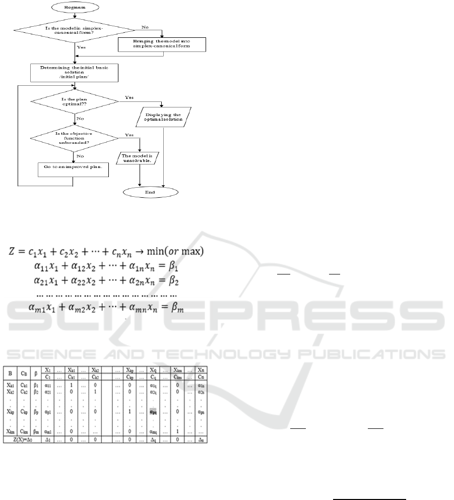
Figure 1: The main stages of solving linear optimization
problems using the Simplex method.
Figure 2: Simplex canonical form.
Table 1: Simplex table.
The first simplex table is filled in. The value of the
objective function and the index estimates are
calculated.
- Z(X) is calculated by multiplying the columns C
B
and β element by element and adding the resulting
products.
- The index estimate Δj of each variable is
calculated by multiplying the column CB element
by element with the column of the variable,
adding the resulting products and subtracting its
target coefficient. The index estimates of the basic
variables are always 0.
Check Optimality
- If the index estimates of all variables are non-
negative ∆

0, 𝑗1,𝑛





, the plan is optimal
when searching maximum value of the objective
function (Z→max) and the algorithm ends.
- If the index estimates of all variables are less than
or equal to zero (∆

0, 𝑗1,𝑛





), the plan is
optimal when searching minimum value
(Z→min) and the algorithm ends.
- If there is an unfavorable index score (Δq) in
whose column there is no positive value (𝛼


0, 𝑖  1, 𝑚






 – the objective function is
unbounded and the model is unsolvable.
- If for each j for which there is an unfavorable
index score Δj there is at least one positive value
in the column, then the plan is not optimal and we
move on to the next plan.
Moving to a neighbour plan
A pivot column is determined – column q, in
which the index score
∆

 is unfavorable. If there are
more than one unfavorable index scores, the more
unfavorable one is selected. The variable of this pillar
becomes the new basic variable in the new plan.
- A pivot row is determined – If exists 𝑖∈

1, 2, … , 𝑚

, for 𝛼

0 which the minimum
ratio (




 min







) is selected.
- Pivot number – the intersection of the pivot row
with the pivot column determines the pivot
number (𝛼

).
- A new simplex table of a neighbor plan is
constructed, in which:
o In columns B and C
B
, only one change is
made - X
kp
is replaced by Xq and C
kp
is
replaced by Cq.
o The elements of the pivot row are divided
by the pivot number.
𝛽


𝛽

𝛼

𝑎𝑛𝑑 𝛼


𝛼

𝛼

, 𝑗  1, 𝑛





1
The remaining values are obtained according to
the rectangle rule (Avramov & Grozev, 2009).
𝛼



𝛼

𝛼

𝛼

𝛼

𝛼

2
From the product of the corresponding element of
the old table with the pivot number is subtracted with
the product of the element from the same row in the
pivot column with the element from the same column
in the pivot row and the result is divided by the pivot
number (Figure 3).
ICEEECS 2025 - International Conference on Advances in Electrical, Electronics, Energy, and Computer Sciences
70

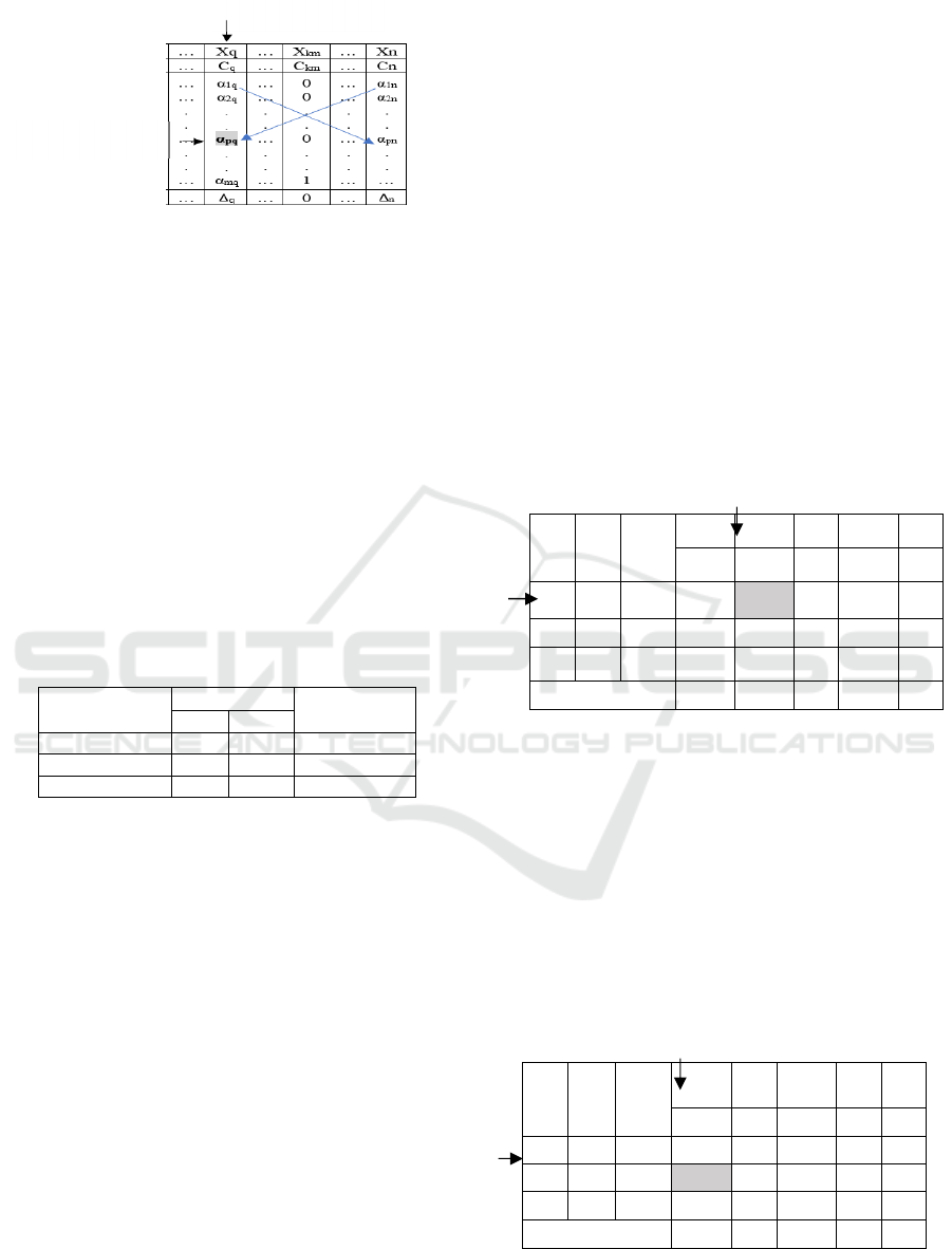
Figure 3: Rectangle rule.
o The value of the objective function and the
index estimates are calculated according to
the rules from step 1 and are proceed to step
2 of the algorithm.
3 RESULTS AND DISCUSSION
3.1 Problem Statement
A company plans to produce two types of products.
Resources required for production are limited,
necessitating optimization. The required resources
per product type and their availability are given in
Table 2.
Table 2: Resource Data
Resource
Item Type
Quantity
А В
Resource 1 2 3 480
Resource 2 4 3 720
Resource 3 3 5 810
How many products of each type should be
produced to obtain maximum profit, if it is known
that the profit from one product of type A is 4 BGN,
and from type B is 5 BGN?
3.2 Solution with Simplex Method
Mathematical description of the problem
- X
1
, X
2
- number of products of type A and B.
- X = (X
1
, X
2
) – production program of the
company and X
1
≥0, X
2
≥0.
- Z – total amount of profit for all manufactured
products. Z= 4X
1
+5X
2
-> max
- The consumption of the three types of resources
for the desired production program X are:
2X
1
+3X
2
≤480
4X
1
+3X
2
≤720
3X
1
+5X
2
≤810
The task of finding a production program of
company is reduced to the following linear
optimization mathematical model:
Z= 4X
1
+5X
2
-> max
2X
1
+3X
2
≤480
4X
1
+3X
2
≤720
3X
1
+5X
2
≤810
X
1
≥0, X
2
≥0
The model is abducted into simplex canonical
form. The initial basis solution is determined.
Z= 4X
1
+5X
2
-> max
2X
1
+3X
2
+X
3
=480
4X
1
+3X
2
+X
4
=720
3X
1
+5X
2
+X
5
=810
X
j
≥0, 𝑗1,5




X
0
(0,0, 480, 720, 810) – the initial basis solution
The model is transferred to the first simplex table
(Table 3).
Table 3: First simplex table
В С
В
β
X
1
X
2
X
3
X
4
X
5
4 5 0 0 0
X
3
0 480 2
3 1 0 0
X
4
07204 3 0 1 0
X
5
0 810 3 5 0 0 1
Z
(0)
=0 -4 -5 0 0 0
Z
(0)
=0.480+0.720+0.810=0
Δ
1
=0.2+0.4+0.3-4=-4
Δ
1
<0 and Δ
2
<0 => The plan is not optimal. The
objective function is checked for unboundedness. The
pivot column, pivot row and pivot number are
determined.
Pivot column – min(Δ
1
, Δ
2
)= Δ
2
Pivot row – min(480/3,720/3,810/5)=480/3
Pivot number – 3
An improved plan is created. A check for
optimality is performed (Table 4).
Table 4: Second simplex table.
В С
В
β
X
1
X
2
X
3
X
4
X
5
4 5 0 0 0
X
2
5 160 2/3 1 1/3 0 0
X
4
0 240 2 0 -1 1 0
X
5
0 10 -1/3 0 -5/3 0 1
Z
(1)
=800 -2/3 0 5/3 0 0
One change is made in columns B and C
B
, by
writing the new basic variable X
2
and its target
Pivot
l
Pivot row
Application of the Simplex Method in Tasks for Determining an Optimal Production Program
71

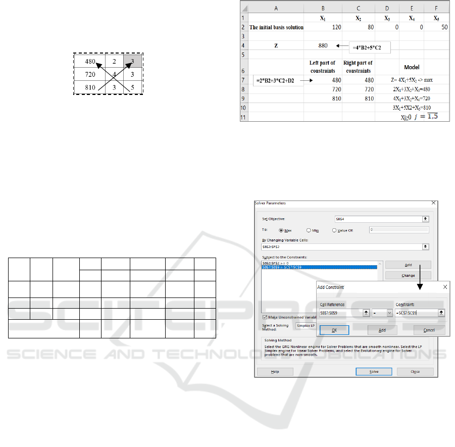
coefficient 5. The row of the new basic variable is
filled in, by dividing the value from the first simplex
table on the pivot number. The remaining values are
calculated according to the rectangle rule (Figure 4).
Figure 4: Rectangle rule.
β
3
=(810.3-5.480)/3=10
Δ
1
<0 => The plan is not optimal. The objective
function is checked for unboundedness. The pivot
column, pivot row and pivot number are determined.
Pivot column – the column of variable X
1
.
Pivot row – the row of variable X
4
.
Pivot number – 2.
An improved plan is created. A check for
optimality is performed (Table 5).
Table 5: Third simplex table.
В С
В
β
X
1
X
2
X
3
X
4
X
5
4 5 0 0 0
X
2
5 80 0 1 2/3 -1/3 0
X
1
4 120 1 0 -1/2 1/2 0
X
5
0 50 0 0 -11/6 1/6 1
Z
(2)
=880 0 0 4/3 1/3 0
Zmax=880, X
1
=120, X
2
=80, X
3
=0, X
4
=0, X
5
=50
The company will realize a maximum profit of
880 BGN when it produces 120 products of type A
and 80 products of type B. In the optimal solution, the
variable X
3
are equal to 0, X
4
is equal to 0, and X
5
is
50. These additional variables that we added to the
model reflect the unused quantities of resources.
Therefore, resources Resource 1 and Resource 2 are
fully used, but there is a rest of 50 units of resource
Resource 3.
3.3 Solution with Solver Tool in
Microsoft Excel
Solving the problem using the Solver tool in
Microsoft Excel requires entering the model into an
Excel worksheet (Figure 5).
Figure 5: Model entered into Microsoft Excel Worksheet
From the Data menu, the Solver tool is selected.
In the Solver Parameters window (Figure 6), the
model parameters are defined.
Figure 6: Model entered into window Solver Parameters.
After running the Solver, the optimal solution is
displayed, allowing the user to save and generate a
report. The optimization algorithm remains hidden
from the user (Ivanova, 2014).
4 CONCLUSIONS
This article presents the algorithm of the simplex
method for solving linear optimization problems. We
explain the theoretical part of the algorithm and
illustrated it in one practically task. The method is
applied to a specific problem related to the
production. This problem we modeled as a linear
optimization problem. We used a simplex method to
find the maximum of the objective function,
respecting all the constraints in the model. The
problem was solved using the Solver tool of
Microsoft Excel also. The Simplex method is
Left
Right
ICEEECS 2025 - International Conference on Advances in Electrical, Electronics, Energy, and Computer Sciences
72

universal, applicable to a wide range of problems in
various fields.
ACKNOWLEDGEMENT
This paper is supported by the Scientific Project
“Integrated Approach for Analysis of Student
Surveys through Statistics and Machine Learning”,
Technical University - Varna, 2025, financed by the
Ministry of Education and Science.
REFERENCES
Ansari, A. (2019). Easy Simplex (AHA Simplex)
algorithm. Journal of Applied Mathematics and
Physics, 7(1), 23–30.
https://doi.org/10.4236/jamp.2019.71003
Anggoro, B., et al. (2019). Profit optimization using
Simplex methods on home industry Bintang Bakery in
Sukarame Bandar Lampung. Journal of Physics:
Conference Series, 1155(1), 012010.
https://doi.org/10.1088/1742-6596/1155/1/012010
Nabli, H. (2009). An overview on the simplex algorithm.
Applied Mathematics and Computation, 210(2), 479–
489. https://doi.org/10.1016/j.amc.2009.01.013
Faculty of Mathematics and Informatics, Sofia University.
(n.d.). Mathematical optimization lecture notes.
Retrieved December 6, 2024, from
https://store.fmi.uni-sofia.bg/fmi/or/MO1/06.pdf
Avramov, A., & Grozev, S. (2009). Matematika (s
prilozheniya v ikonomikata i biznesa) [Mathematics
with applications in economics and business]. Tsenov
Academic Publishing House.
Ivanova, M. (2014). Reshavane na zadachi ot lineynata
algebra i lineynoto optimirane s pomoshtta na MS
Excel [Solving problems in linear algebra and linear
optimization with the help of MS Excel]. Ikonomicheski
i sotsialni alternativi, 1, 20–29.
Application of the Simplex Method in Tasks for Determining an Optimal Production Program
73