Comparison of Linear Regression, MLP, 1D CNN, and Graph Neural

Networks for Financial Asset Forecasting

Xiaoting Yang

Computer Science, University of Wisconsin-Eau Claire, Eau Claire, Wisconsin, U.S.A.

Keywords: Financial Time Series, Stock Price Forecasting, Deep Learning Models, Graph Neural Networks, SHAP

Interpretability.

Abstract: Recent advances in deep learning have led to powerful new tools for modeling complex, nonlinear patterns

in financial markets. This study conducts a head-to-head comparison of four distinct forecasting approaches—

linear regression, multilayer perceptron (MLP), one-dimensional convolutional neural network (1D CNN),

and graph neural network (GNN)—to predict next-day adjusted closing prices for two equities (Amazon and

Netflix), one consumer-goods stock (Domino’s Pizza), and one cryptocurrency (Bitcoin). The results

demonstrate that while all four methods achieve similarly high accuracy on the more stable equity series (R²

≈ 0.96–0.97), the nonlinear neural models—particularly the MLP and 1D CNN—offer clear advantages for

the highly volatile Bitcoin series (R² ≈ 0.92–0.93 compared to ≈ 0.86–0.88 for the linear and graph-based

models). To shed light on each model’s decision process, this paper employ SHapley Additive exPlanations

(SHAP) and find that the most recent price lag (the prior day’s close) consistently carries the greatest

predictive weight across all methods. These findings highlight both the strengths and limitations of deep

learning approaches in one-step financial forecasting and underscore the value of interpretability techniques

for understanding model behavior.

1 INTRODUCTION

Financial time series forecasting, including stock and

cryptocurrency price prediction, is a crucial but

challenging field. Accurate forecasts can inform

investment decisions, but market dynamics are non-

stationary and often volatile. Traditional statistical

methods have been used but struggle with nonlinear

patterns and abrupt shifts. Recent surveys note that

deep learning has emerged as a “new frontier” in stock

market forecasting, and that data-driven neural

networks have become mainstream in financial

prediction. Deep learning has recently seen extensive

application in stock market prediction, with

significant advancements being continually achieved

in terms of forecast accuracy and robustness (Jiang,

2021; Bao et al., 2025)

Among machine learning models, feedforward

networks like MLP serve as flexible nonlinear

regressors, while specialized architectures capture

temporal structure. CNN applies convolutional filters

along the time axis to extract local features from price

https://orcid.org/0009-0008-9189-7277

sequences. For example, Zeng emphasize that CNNs

effectively capture short-term dependencies in

financial series. Recurrent models (e.g., LSTM, GRU)

capture longer-term sequential dependencies, though

they may still miss complex multi-asset interactions

(Zeng et al., 2023). Zhang review notes that deep

learning models are increasingly favored over

traditional ones for price forecasting. These

approaches can model nonlinear relationships that

simple models cannot (Zhang et al., 2023).

Graph Neural Networks (GNNs) have emerged

prominently in recent years, widely applied to node

classification, link prediction, and graph classification

tasks, demonstrating strong modeling capabilities

across various domains (Zhou et al., 2021; Wu et al.,

2020). GNNs explicitly leverage graph structure. In a

GNN, each data point is a node, and edges encode

relationships, enabling information to propagate

across the graph. In finance, one can represent each

time step as a node or each asset as a node. Surveys by

Jin note that GNNs can model inter-temporal and

inter-variable relationships that standard methods

struggle to capture (Jin et al., 2024). For instance, Ran

Yang, X.

Comparison of Linear Regression, MLP, 1D CNN, and Graph Neural Networks for Financial Asset Forecasting.

DOI: 10.5220/0014321000004718

Paper published under CC license (CC BY-NC-ND 4.0)

In Proceedings of the 2nd International Conference on Engineering Management, Information Technology and Intelligence (EMITI 2025), pages 84-91

ISBN: 978-989-758-792-4

applied graph convolution on a stock-correlation

graph and reported improved trend predictions (Ran et

al., 2024). These studies suggest that GNNs leverage

structural information beyond what feedforward or

convolutional networks capture.

Interpretability is also essential. Complex models

can be opaque, so explainable AI tools highlight the

importance of features. SHAP assigns each input

feature an importance value for a prediction. Dost et

al. applied SHAP to a stock trend model and identified

the features driving its predictions (Muhammad et al.,

2024). SHAP is widely adopted as a model

interpretability technique due to its clear and intuitive

feature importance explanations and has become a

standard tool in explainable machine learning

(Lundberg & Lee, 2017). My study uses SHAP to

interpret how each model weighs input price features.

This study systematically compares Linear

Regression, MLP, 1D CNN, and GNN on identical

datasets for four assets (Amazon, Domino’s Pizza,

Bitcoin, and Netflix). Each model is trained on

historical adjusted closing prices (May 2013–May

2019) and evaluated on held-out test data. Forecast

accuracy is measured by the coefficient of

determination (R²), and the research visualize

predicted vs. actual price trajectories. The research

also computes SHAP values to analyze the importance

of each model's feature. The goal is to understand the

strengths and limitations of each model class in

financial time series forecasting.

2 DATASET AND

METHODOLOGY

2.1 Dataset

Historical daily price data for AMZN, DPZ, BTC, and

NFLX were obtained from Kaggle. The period covers

May 2013 through May 2019, yielding roughly 1500

trading days per asset. The dataset includes columns

Open, High, Low, Close, Adjusted Close, and

Volume. This research focuses on the Adjusted Close

price as the primary series for forecasting. The data

were split chronologically: the first 70% of records

are used for training and the last 30% for testing. All

price features were normalized to the range [0,1] to

aid model training.

2.2 Methods

As shown in Figure 1, Linear Regression is an

ordinary least squares model that predicts the next-

day price as a linear combination of input features.

The research uses a fixed number of past days as input

features. Linear regression provides a simple,

interpretable baseline that captures linear trends in the

data.

Figure 1: Linear Regression (Picture credit: Original).

As shown in Figure 2, MLP: A fully connected

feedforward neural network. The MLP takes a fixed

window of past prices as input, processes them

through one or more hidden layers with ReLU

activation, and outputs the predicted next price. The

research trains the network via backpropagation using

mean squared error loss. The MLP can learn complex

nonlinear mappings from the input history to future

prices.

As shown in Figure 3, 1D CNN: A convolutional

network that applies one-dimensional convolution

filters along the time axis of the input window. The

CNN extracts local temporal features via successive

convolutional layers before a final fully connected

output. 1D CNNs effectively capture local trends and

patterns in time series. CNN architecture uses several

convolutional layers to process the input window and

then regresses to the next-day price.

Figure 2: MLP (Picture credit: Original).

Figure 3: 1D CNN (Picture credit: Original).

Comparison of Linear Regression, MLP, 1D CNN, and Graph Neural Networks for Financial Asset Forecasting

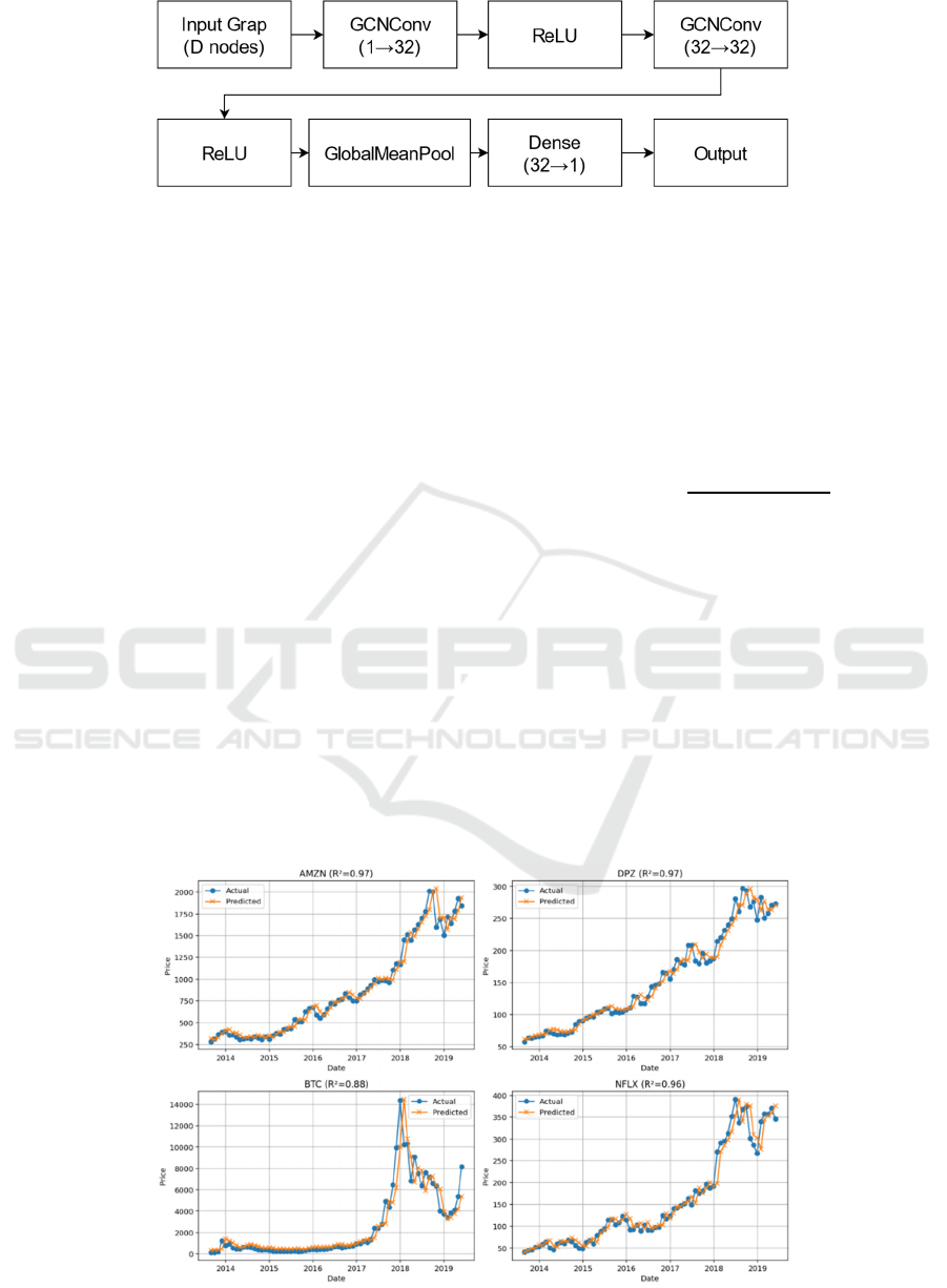
Figure 3: GNN (Picture credit: Original).

As shown in Figure 4, GNN have emerged

prominently in recent years, widely applied to node

classification, link prediction, and graph

classification tasks, demonstrating strong modeling

capabilities across various domains (Zhou et al.,

2021; Wu et al., 2020). The research constructs a

graph for each time series where each node represents

a day’s data. Edges connect consecutive days,

forming a chain graph. The GNN applies graph

convolution or message-passing layers: each node

updates its embedding by aggregating information

from its neighbors. After graph convolution, the

research uses a readout layer to predict the next-day

price from the final node features. This architecture

allows the model to learn patterns across adjacent

time points.The objective for all models is to predict

the next day Adjusted Close price. The research trains

each model on the training set and evaluate

performance on the test set. After training, the

research applied SHAP to each model to measure the

importance of each feature. SHAP computes a

contribution value for each input feature in each

prediction, which helps interpret how each past price

contributes to the forecast.

3 EXPERIMENTS

3.1 Evaluation Metric

The research evaluates forecasting accuracy using the

coefficient of determination, R². The R² score is

defined as:

𝑅



1

∑





,



,







∑





,











(1)

where y_(true,i) are the actual prices, y_(pred,i) are

the predicted prices, and y ̅ is the mean of the actual

prices in the test set. An R² of 1.0 indicates perfect

prediction, while 0 indicates the model explains none

of the variance. The research report R² on the test set

for each model and asset.

3.2 Results

As shown in Figure 5, the linear regression model

forecasts (orange) versus actual prices (blue) for

AMZN, DPZ, BTC, and NFLX are shown above.

Linear

regression achieved R²≈0.97 for AMZN

Figure 4: Linear Regression Results (Picture credit: Original).

EMITI 2025 - International Conference on Engineering Management, Information Technology and Intelligence

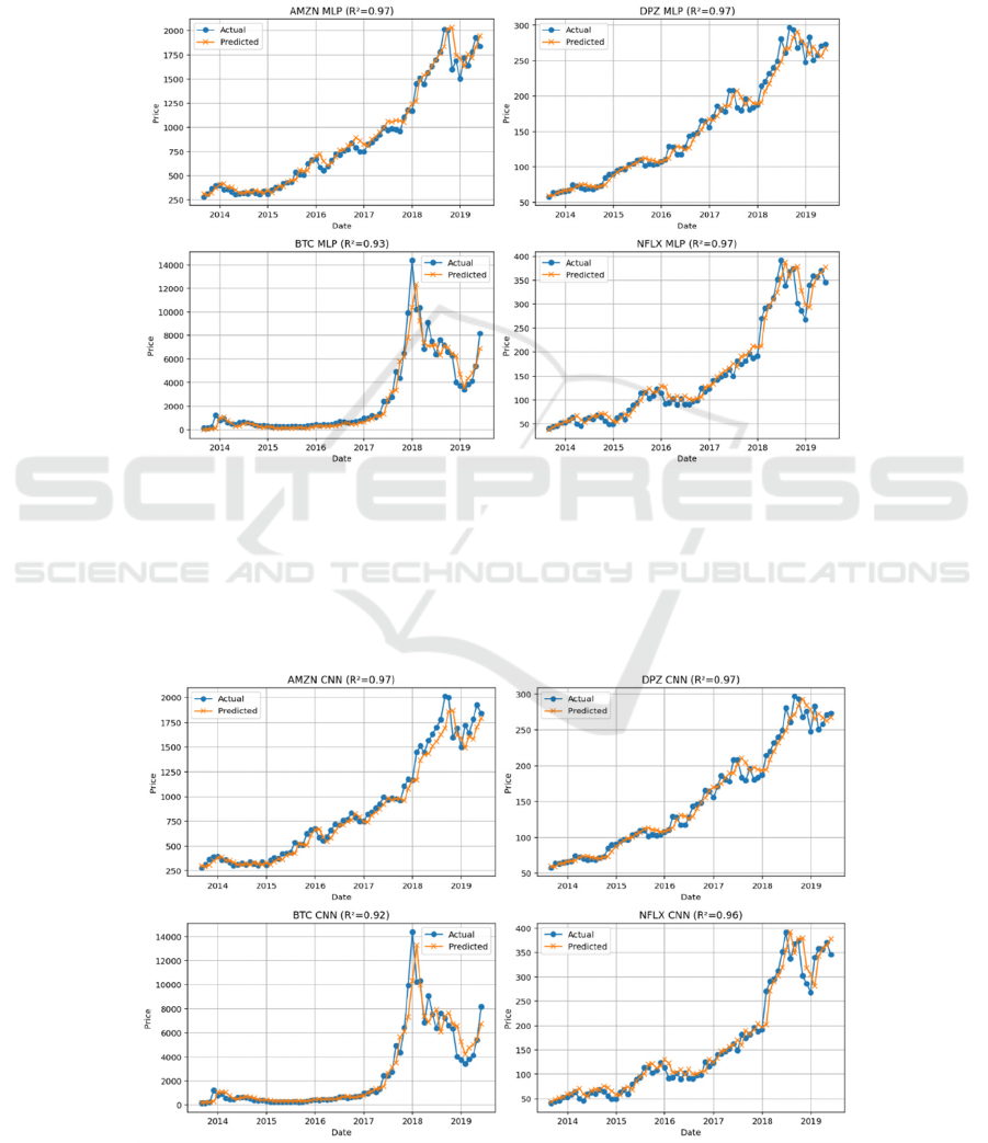
and DPZ, and R²≈0.96 for NFLX, indicating accurate

fits on these stocks. Bitcoin’s forecast is less precise

with R²≈0.88. The plot shows that the linear model

tracks the long-term trends in the stock prices well,

but it underestimates the rapid spikes in Bitcoin.

The Figure 6 above displays the MLP results. The

MLP attains R²≈0.97 for AMZN, DPZ, and NFLX.

For BTC, the MLP achieves a higher R²≈ 0.93,

outperforming the linear model. The predictions

(orange) closely follow most of each series' actual

(blue). In particular, the MLP’s nonlinear learning

allows it to capture Bitcoin’s volatility more

effectively, as seen by the tighter fit to the large BTC

price swings.

Figure 5: MLP Results (Picture credit: Original).

As shown in Figure 7, the CNN also achieves R²≈

0.97 for AMZN and DPZ, and R²≈0.96 for NFLX,

like the other models. For BTC, the CNN’s R²≈0.92,

slightly lower than the MLP but higher than linear

regression. The CNN predictions (orange) capture

many of the local fluctuations in each series. The

CNN’s performance is comparable to the MLP,

successfully learning short-term patterns in the time

series.

Figure 6: 1D CNN Results (Picture credit: Original).

Comparison of Linear Regression, MLP, 1D CNN, and Graph Neural Networks for Financial Asset Forecasting

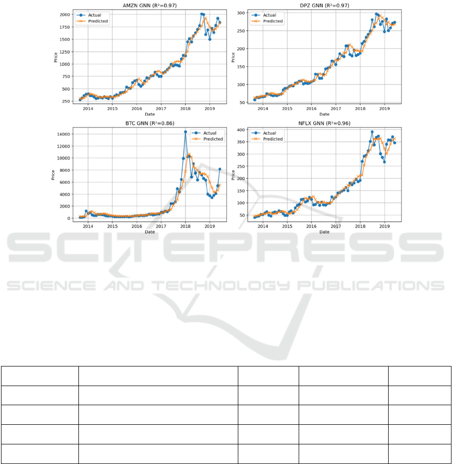
As shown in Figure 8, the GNN achieves R²≈0.97

for AMZN and DPZ, and R²≈0.96 for NFLX, again

on par with the other stock models. However, for

BTC, the GNN’s R²≈0.86 is the lowest. The predicted

Bitcoin prices (orange) show larger deviations from

actual (blue) at peak points. This suggests that the

simple graph construction did not improve Bitcoin

forecasting. The GNN performed similarly to linear

regression on BTC but did not capture its extreme

moves.

Figure 7: GNN Results (Picture credit: Original).

As shown in Table 1, all models fit the stock price

data well (R² ≈ 0.96–0.97). The main performance

differences occur on Bitcoin: the MLP and CNN

achieved higher R² ( ≈ 0.92–0.93) than Linear

Regression (0.88) or the GNN (0.86). This indicates

that the neural networks’ nonlinear modeling helped

capture Bitcoin’s volatility. Nevertheless, even the

lowest R² (0.86) still represents a reasonable fit.

Visually, the predicted and actual prices mostly align

across all assets. Thus, the deeper models provided

marginal gains on stocks but offered noticeable

improvement for the highly volatile cryptocurrency.

Table 1: Comparison of Forecasting Performance (R² values) Across Models and Assets.

Asset Linear Regression MLP 1D CNN GNN

AMZN 0.97 0.97 0.97 0.97

DPZ 0.97 0.97 0.97 0.97

NFLX 0.96 0.97 0.96 0.96

BTC 0.88 0.93 0.92 0.86

3.3 Feature Important Analysis

As shown in Figure 9, it relies most on the previous

day's closing price (Price_t-1), followed by the price

of the last 5 days (Price_t-5). This shows that the

short-term (one day) and slightly longer lagged (five

days) prices of AMZN have the most influence on the

prediction, while the importance of the middle days is

relatively low.

EMITI 2025 - International Conference on Engineering Management, Information Technology and Intelligence

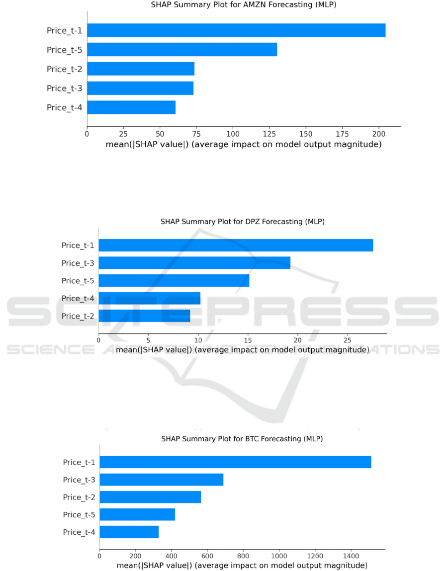
Figure 9: AMZN prediction (Picture credit: Original).

As shown in Figure 10, like AMZN, Price_t-1 still

has the highest importance, followed by Price_t-3 and

Price_t-5. This indicates that the prediction of DPZ

price is significantly affected by recent (1 day ago)

and slightly distant (3 days and 5 days ago) price

information.

Figure 10: DPZ prediction (Picture credit: Original).

As shown in Figure 11, BTC's price fluctuates

violently. SHAP analysis shows that the closing price

of the previous day (Price_t-1) has a very high impact

on BTC prediction, far greater than other lagged

features. The importance of other features (Price_t-3,

Price_t-2, Price_t-5, Price_t-4) decreases in turn,

indicating that the model's prediction of BTC mainly

relies on extremely short-term price information.

Figure 11: BTC prediction (Picture credit: Original).

Comparison of Linear Regression, MLP, 1D CNN, and Graph Neural Networks for Financial Asset Forecasting

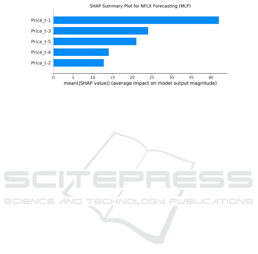
Figure 12: NFLX prediction (Picture credit: Original).

As shown in Figure 12, the SHAP analysis results

of NFLX also show that the price of the previous day

(Price_t-1) is the most important, followed by the last

3 days (Price_t-3) and the previous 5 days (Price_t-

5). This is like the situation of DPZ, indicating that

NFLX predictions strongly rely on historical price

information from recent and past days.

In summary, the feature importance analysis of

the four assets shows that the MLP model generally

relies heavily on the most recent one-day price

information (Price_t-1) when predicting future prices

and then selectively refers to other lagged days of

prices based on the characteristics of different assets.

This reflects that the model can capture the price

volatility characteristics of different assets.

4 CONCLUSIONS

In the experiments, all models achieved high

accuracy on the stock assets (AMZN, DPZ, NFLX),

with R² values around 0.96–0.97. The simpler Linear

Regression baseline performed nearly as well as the

neural models on these well-behaved series.

However, the neural models outperformed for the

volatile cryptocurrency: the MLP and CNN achieved

the highest R² (≈0.92–0.93) while Linear Regression

and the GNN were lower (≈0.86–0.88). This indicates

that the nonlinear learning capacity of the MLP and

CNN helps capture Bitcoin’s erratic behavior better

than the linear model or the GNN.

SHAP analysis revealed that, for each model, the

most recent price lags were the dominant features

influencing predictions. This confirms that all models

rely primarily on immediate price history in one-step

forecasting. Overall, deeper models provided only

marginal gains on stable stock forecasts but delivered

more benefit on the highly volatile asset.

This study has limitations. We used only historical

adjusted closing prices as inputs to predict next day

closing prices, without incorporating additional

potentially influential variables such as

macroeconomic factors, or market sentiment data.

Including these additional features could enhance

predictive performance. Furthermore, the graph

construction for the GNN was relatively

straightforward, utilizing only temporal relationships

within individual assets; constructing more complex,

multi-asset interaction graphs might further improve

forecasting accuracy. Additionally, this research

focused exclusively on one-step-ahead predictions

evaluated via the R² metric; future studies could

extend analyses to multi-day forecasts, employ

alternative evaluation metrics, and explore more

sophisticated neural network architectures. Despite

these limitations, the study provides a comprehensive

comparison among predictive models and highlights

the importance of interpretability in financial time

series forecasting.

REFERENCES

Bao, W., Cao, Y., Yang, Y., Che, H., Huang, J., Wen, S.,

… Zhang, C. (2025). Data-driven stock forecasting

models based on neural networks: A review.

Information Fusion, 113, 102616.

Graph neural networks: A review of methods and

applications. AI Open, 1, 57–81.

Jiang, W. (2021). Applications of deep learning in stock

market prediction: Recent progress. Expert Systems

with Applications, 184, 115537.

Jin, M., Koh, H. Y., Wen, Q., Zambon, D., Alippi, C.,

Webb, G. I., & Pan, S. (2024). A survey on graph neural

EMITI 2025 - International Conference on Engineering Management, Information Technology and Intelligence

networks for time series: Forecasting, classification,

imputation, and anomaly detection. arXiv preprint

arXiv:2307.03759.

Lundberg, S. M., & Lee, S.-I. (2017). A unified approach

to interpreting model predictions. In Advances in

Neural Information Processing Systems, 30.

Muhammad, D., Ahmed, I., Naveed, K., Bendechache, M.,

& Yaseen, U. (2024). An explainable deep learning

approach for stock market trend prediction. Heliyon,

10(21), e40095.

Ran, Y., Fan, Y., Wang, Y., Yu, Z., & Han, J. (2024). A

model based on LSTM and graph convolutional

network for stock trend prediction. PeerJ Computer

Science, 10, e518.

Wu, Z., Pan, S., Chen, F., Long, G., Zhang, C., & Yu, P. S.

(2020). A comprehensive survey on graph neural

networks. IEEE Transactions on Neural Networks and

Learning Systems, 32(1), 4–24.

Zeng, Z., Kaur, R., Siddagangappa, S., Rahimi, S., Balch,

T., & Veloso, M. (2023). Financial time series

forecasting using CNN and Transformer. arXiv preprint

arXiv:2304.04912.

Zhang, C., Sjarif, N. N. A., & Ibrahim, R. (2023). Deep

learning models for price forecasting of financial time

series: A review of recent advancements (2020–2022).

arXiv preprint arXiv:2305.04811.

Zhou, J., Cui, G., Hu, S., Zhang, Z., Yang, C., Liu, Z.,

Wang, L., & Sun, M. (2021).

Comparison of Linear Regression, MLP, 1D CNN, and Graph Neural Networks for Financial Asset Forecasting