Data Complexity-Oriented Classification of Multispectral Remote

Sensing Imagery via Machine and Deep Learning Approaches

Berrin Islek

and Hamza Erol

Department of Computer Engineering, Sivas Science and Technology University, Sivas, Turkey

Department of Computer Engineering, Mersin University, Mersin, Turkey

Keywords: Deep Neural Network, Data Complexity, Computational Complexity, Information Complexity, Support

Vector Machines, Random Forest.

Abstract: In this study, the land cover of an agricultural region was classified at a field level using multispectral satellite

imagery. The primary objective of the study was to evaluate different classification methods in terms of data

complexity, computational complexity, and information complexity. The data labelling process was

performed using hierarchical clustering, making the groups in the data more meaningful. A separate clustering

tree structure was created for each feature, and data complexity was analysed using parameters such as level,

number of families, and number of children. Object-oriented approaches were adopted in the classification

phase, employing Deep Neural Networks, Random Forest, and Support Vector Machines. The performance

of these methods was examined not only in terms of accuracy but also in terms of evaluation metrics such as

F1-score, recall, and precision. The results demonstrate the classification capabilities of the methods in a

comprehensive manner and provide important clues about which approach is more suitable in different

scenarios. Furthermore, the methods were compared in terms of computational costs and processing times,

and a comprehensive evaluation was conducted regarding the classification of agricultural regions using

remotely sensed data.

1 INTRODUCTION

Multispectral remote sensing images are widely used

to classify vegetation types and estimate crop yields

in agricultural regions (Thyagharajan and Vignesh,

2019; Modica et al., 2021). This approach has

emerged as a key resource in contemporary precision

agriculture, allowing extensive assessment of crop

conditions, vegetation patterns, and soil

characteristics (Sishodia et al., 2020; Guanter et al.,

2013). These images capture data across multiple

spectral bands, providing information that is not

visible to the human eye, which is crucial for accurate

assessment of crop status and yield prediction

(Thenkabail, Lyon, & Huete, 2016).

Over the years, various approaches have been

proposed to improve classification accuracy using

multispectral images. For example, Erol and Akdeniz

employed mixture distribution models for land cover

classification, achieving an accuracy of 94% (Erol &

https://orcid.org/ 0000-0003-1984-357X

https://orcid.org/0000-0001-8983-4797

Akdeniz, 2005). Sehgal applied preprocessing

techniques and different classification algorithms to

multispectral satellite images, reaching a maximum

accuracy of 87% using a Backpropagation Neural

Network (BPNN) (Sehgal, 2012). Similarly, Çalış

and Erol (2012) applied mixture discriminant

analysis, while Crnojević et al. (2014) integrated

Landsat-8 and RapidEye images for pixel-based

classification in northern Serbia. Gogebakan and Erol

(2018) developed a semi-supervised approach for

classifying multispectral data, which utilizes

clustering based on mixture models. Sicre et al.

(2020) analyzed the contribution of microwave and

optical data for land type classification in

southwestern France, achieving up to 85% accuracy

using Support Vector Machines and Random Forests.

Selecting an appropriate classification method for

multispectral satellite imagery of agricultural regions

containing diverse crop types remains a critical task.

To address this challenge, numerous machine

Islek, B. and Erol, H.

Data Complexity-Oriented Classiﬁcation of Multispectral Remote Sensing Imagery via Machine and Deep Learning Approaches.

DOI: 10.5220/0014313500004848

Paper published under CC license (CC BY-NC-ND 4.0)

In Proceedings of the 2nd International Conference on Advances in Electrical, Electronics, Energy, and Computer Sciences (ICEEECS 2025), pages 257-265

ISBN: 978-989-758-783-2

257

learning and deep learning algorithms have been

developed to improve land use and vegetation

classification accuracy. In Dash et al. (2023) study,

LandSat image data was used to increase the accuracy

of land use and vegetation classification in

agricultural regions. In this study, Support Vector

Machines (SVM) (Kadavi & Lee, 2018; Singh,

Gayathri, & Chaudhuri, 2022), Random Forest

Classifier (RFC) (Pal, 2005; Zhang et al., 2017), and

Deep Neural Networks (DNN) (Singh et al., 2025)

were used. The objectives of this study are as follows:

First, the complexity of remotely sensed multi-

spectral satellite imagery will be calculated and data

labeling will be performed. Then, we will classify

remotely sensed multi-spectral satellite imagery of

agricultural regions using object-based SVM, RFC,

and DNN classification methods and compare the

classification performance of these three methods.

Finally, the obtained results will be evaluated and

discussed.

2 MATERIALS AND METHOD

In this section, we provide a comprehensive

description of the study workflow. Specifically, we

discuss (i) the remotely sensed multispectral images

of the agricultural region under study, (ii) the

complexity of these data, (iii) the data labelling

process, (iv) the classification methods applied to

these datasets, and (v) the performance evaluation

metrics used to assess the models.

2.1 Remotely Sensed Multispectral

Image of Agricultural Region

The multispectral imagery employed in this research

was obtained using the Landsat Thematic Mapper and

depicts an agricultural region situated in the Seyhan

Plain (approximately 37° N, 36° E) in Adana, Turkey.

The image spans an area of 198 × 200 pixels, resulting

in a total of 39,600 pixels, and was acquired on 27

March 1992 (Path 175–Row 34). For analysis, bands

3, 4, and 5 were selected, as they are effective in

differentiating healthy vegetation, open water, and

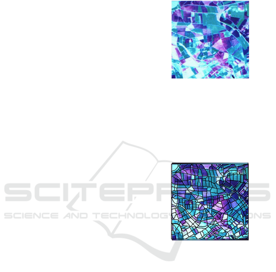
soil surfaces, respectively. Figure 1 presents the

Landsat Thematic Mapper image of the study area

without incorporating prior field information.

Figure 1: Landsat Thematic Mapper image, without a prior

information, of the agricultural region studied.

The study area consists of 269 individual fields,

labeled with codes from F001 to F269 on the

parcelization map prepared by the Government

Irrigation Department (DSI). Five major land cover

classes—wheat, potato, vegetable garden, citrus, and

bare soil—are present in the region, with a total of 24

subcategories. Based on this classification, 24 control

fields have been defined within the area.

Figure 2: Landsat Thematic Mapper image of the study

area, incorporating the previously collected parcel

information.

Based on a land cover survey, the control plots

were designated with identifiers CF001 to CF024 on

the parcel map provided by the Government Irrigation

Department. The remaining 245 plots, serving as test

sites, were labeled TF001 through TF245 on the same

map. Figure 2 shows a Landsat Thematic Mapper

image of the study area, incorporating the previously

collected parcel information.

2.2 Data Complexity Analysis of

Multispectral Remote Sensing

Image in Agricultural Regions

The multispectral image data analysed in this study

were acquired using the Landsat Thematic Mapper

sensor. Let’s bands 3, 4 and 5 values denoted by

ICEEECS 2025 - International Conference on Advances in Electrical, Electronics, Energy, and Computer Sciences

258

variables X

, X

and X

respectively. There are 39600

instances (observations) surrounding 198x200 data

matrix for each variable (feature).

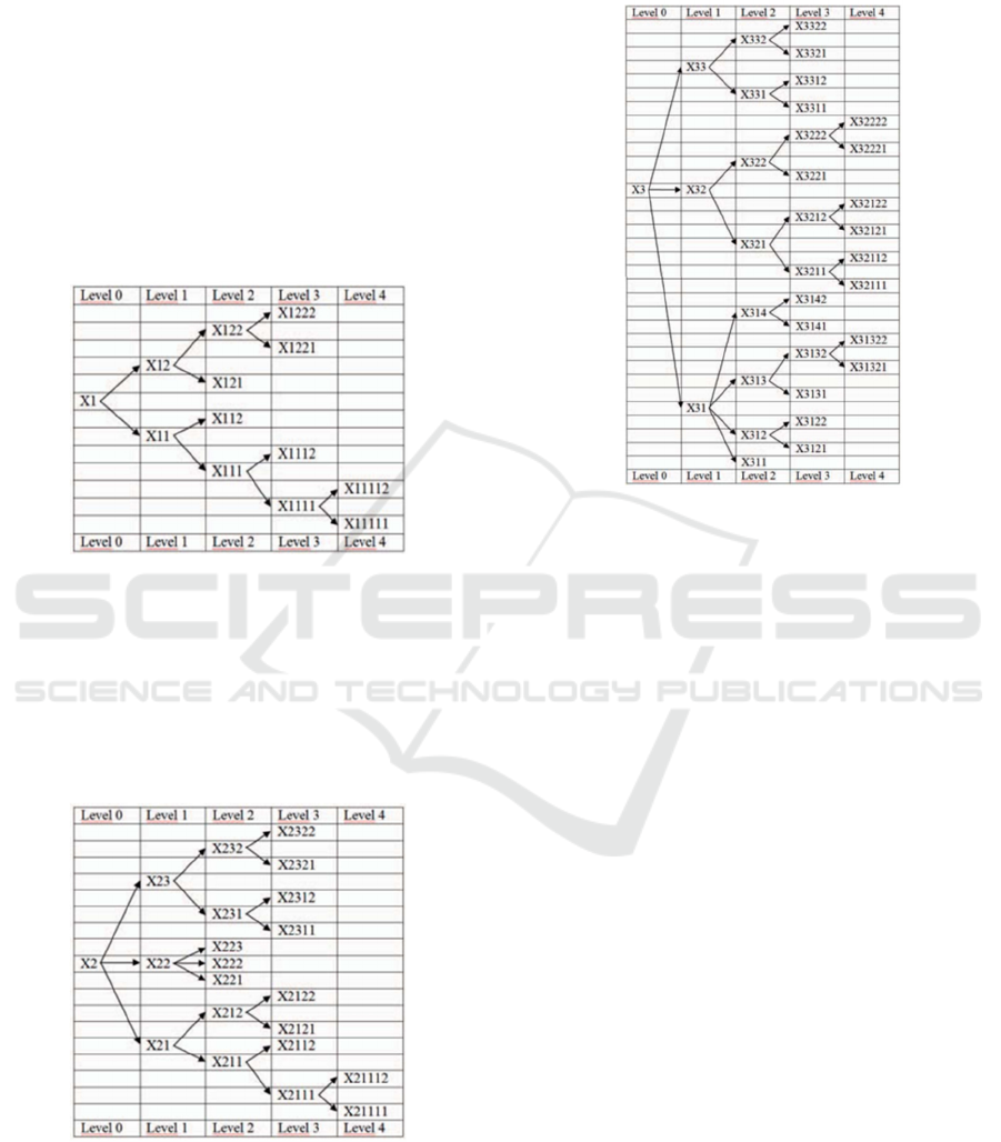
The method for determining the degree of data

complexity is based on hierarchical structure of all

groups and all clusters in data (Erol & Erol, 2018).

The assessment of data complexity is conducted by

utilizing the hierarchical tree structure of groups and

clusters based on the features of the data. The tree

structures are obtained by finding all groups for each

feature in data. The hierarchical tree structures of all

groups in each feature for obtaining remotely sensed

multispectral image data complexity were shown in

Fig. 3 – Fig. 5 respectively.

Figure 3: The hierarchical tree structures of all groups in the

first feature X

for remotely sensed multispectral image

data complexity.

The number of levels is 4, the number of parent

nodes (npn

) is 5 and the number of child nodes (ncn

)

is 7 in hierarchical tree structures of all groups in

feature X

for remotely sensed multispectral image

data as shown in Fig 3 (Erol & Erol, 2018).

Figure 4: The hierarchical tree structures of all groups in the

second feature X

for remotely sensed multispectral image

data complexity.

The number of levels is 4, the number of parent

nodes (npn

) is 8 and the number of child nodes (ncn

)

is 12 in hierarchical tree structures of all groups in

feature X

for remotely sensed multispectral image

data as shown in Fig 4 (Erol & Erol, 2018).

Figure 5: The hierarchical tree structures of all groups in the

third feature X

for remotely sensed multispectral image

data complexity.

The number of levels is 4, the number of parent

nodes (npn

) is 14 and the number of child nodes

(ncn

) is 19 in hierarchical tree structures of all groups

in feature X

for remotely sensed multispectral image

data as shown in Fig 5 [18].

Let ncn

and npn

denote the number of child

nodes and parent nodes for feature X

respectively.

Let DCX

denote data complexity for feature X

. Then

the data complexity for each feature X

is defined as

DCX

= ncn

- npn

for i=1,2,3 (1

)

So DCX

= 2, DCX

= 4 and DCX

= 5 for i=1,2,3

respectively. Let DC denote the data complexity for

entire data. Thus for all features. Then DC is defined

as:

DC =

∏

DCX





)

DCX

= 2, DCX

= 4 and DCX

= 5 for feature

, X

and X

are 2, 4 and 5 respectively. Then the

data complexity for entire data DC = DCX

* DCX

= 2 * 4 * 5 = 40. In the rest of this study, with

this DC = 40 for entire data which classification

method among three methods give the best

classification performance will be determined. Thus,

which method? Machine learning methods versus

deep learning method.

Data Complexity-Oriented Classiﬁcation of Multispectral Remote Sensing Imagery via Machine and Deep Learning Approaches

259

2.3 Data Labelling of Remotely

Acquired Images for Agricultural

Lands

Two types of data are considered in this study:

incomplete data, which lack class labels, and

complete data, which include class labels. Class

labels (or class codes) are essential for the

classification of vector data. For the remotely sensed

multispectral image data of the agricultural area, data

labelling was performed based on the field (parcel)

structure within the region. A total of 245 test fields

and 24 control fields were identified in the

multispectral imagery using an edge detection

algorithm in conjunction with the parcelization map

of the agricultural area. The field types and

corresponding class codes are listed in Table 1.

Table 1: Control field codes and data labels (class codes).

Field Types Data Labels

Wheat1 1

Wheat2 2

Wheat3 3

Wheat4 4

Wheat5 5

Wheat6 6

Potato1 7

Potato2 8

Potato3 9

Potato4 10

Vegetable garden1 11

Vegetable garden2 12

Vegetable garden3 13

Vegetable garden4 14

Vegetable garden5 15

Vegetable garden6 16

Citrus1 17

Citrus2 18

Citrus3 19

Citrus4 20

Bare soil1 21

Bare soil2 22

Bare soil3 23

Bare soil4 24

Bare soil5 25

Data labelling is made for totally 39600 instances

(observations) in the 245 test fields and 24 control

fields of remotely sensed multispectral image data in

the agricultural area. Complete data is obtained as

comma separated values data file.

2.4 Classification Methods

The Support Vector Machine (SVM) is a supervised

learning algorithm grounded in Vapnik’s statistical

learning theory (Vapnik, 2013). Its main objective is

to identify the optimal separation boundaries between

classes. By using a kernel function, SVM can project

training examples into a higher-dimensional space,

allowing it to distinguish classes that are not linearly

separable in the original feature space. The selection

of the kernel function is a key design choice. Typical

kernels include linear, polynomial, radial basis

function (RBF), and sigmoid. In this study, the RBF

kernel is chosen because of its effectiveness in

managing non-linear separation tasks (Kadavi & Lee,

2018).

The Random Forest Classifier (RFC) is an

ensemble learning technique that generates a

collection of decision trees, each trained on randomly

selected subsets of data and features. At every split

within a tree, only a randomly chosen portion of the

available attributes is considered for determining the

division (Breiman, 1999). Each tree produces its own

prediction for a given input, and the final

classification outcome is obtained through majority

voting across the ensemble. This approach improves

model stability and helps mitigate overfitting. For the

induction of individual decision trees, a feature

selection criterion and a pruning strategy must be

specified. Among the available criteria, the Gini

index is widely used to select the most informative

feature at each split. The aggregation of predictions

from the N randomly constructed trees forms the

foundation of the Random Forest algorithm.

Subsequently, the trained forest is used to predict the

labels of samples in the test dataset, and the class with

the most votes across the trees is assigned as the final

prediction (Pal, 2005).

A Deep Neural Network (DNN) is an advanced

type of artificial neural network designed to capture

complex relationships in data through multiple layers

of interconnected neurons. Inspired by the

information processing mechanisms of the human

brain, DNNs consist of several hidden layers, where

each layer transforms the output of the previous layer

into increasingly abstract representations. Training

typically involves the backpropagation algorithm,

which adjusts network weights by propagating

prediction errors backward, allowing the network to

improve its performance iteratively. The

effectiveness of a DNN depends on several factors,

including structural choices such as the number of

layers and neurons per layer, learning parameters

such as activation functions, learning rate, number of

ICEEECS 2025 - International Conference on Advances in Electrical, Electronics, Energy, and Computer Sciences

260

epochs, batch size, and the use of regularization

methods. These factors collectively influence how

well the network learns patterns, generalizes unseen

data, and avoids overfitting. DNNs are particularly

suitable for handling large-scale and high-

dimensional datasets due to their capacity for

hierarchical feature extraction (Schmidhuber, 2014).

2.5 Performance Measures

Evaluating classification models requires not only the

correct implementation of algorithms but also the

selection of appropriate performance metrics. These

metrics quantify how well a model predicts class

labels and help identify which aspects of performance

are most relevant for a given application. For

balanced datasets, accuracy may provide a sufficient

measure, whereas for imbalanced datasets, precision,

recall, and F1-score offer more informative

assessments. Therefore, multiple metrics are typically

reported rather than relying on a single measure.

In classification tasks, the performance of a model

is commonly evaluated by comparing its predicted

labels with the actual labels. These results can be

summarized in a confusion matrix, which presents the

counts of correctly and incorrectly classified samples.

Instances that are correctly predicted as positive are

referred to as True Positives (TP), whereas correctly

predicted negative instances are True Negatives (TN).

False Positives (FP) indicate negative cases that were

mistakenly classified as positive, and False Negatives

(FN) represent positive cases incorrectly identified as

negative. These counts serve as the basis for

computing various performance metrics.

Accuracy, for example, quantifies the ratio of

correctly classified samples to the total number of

observations. (see Eq. 3)

𝐴

𝑐𝑐𝑢𝑟𝑎𝑐𝑦 =





(3)

Precision indicates the fraction of predicted

positive instances that are actually positive, reflecting

the model’s reliability in its positive predictions. (see

Eq. 4)

𝑃𝑟𝑒𝑐𝑖𝑠𝑖𝑜𝑛 =

TP + FP

(4)

Recall, also referred to as sensitivity, measures the

fraction of actual positive instances that the model

successfully identifies, capturing its ability to detect

positive cases. (see Eq. 5)

𝑅𝑒𝑐𝑎𝑙𝑙 =

(5)

The F1-score provides a balanced assessment by

combining precision and recall through their

harmonic mean, offering a single measure that

considers both false positives and false negatives.

(see Eq. 6) (Dalianis, 2018)

𝐹1 𝑠𝑐𝑜𝑟𝑒 = 2 ∗

∗



)

These metrics together offer a comprehensive

evaluation of classification performance and were

used to assess the predictive models in this study.

3 RESULTS

In this section, all classification experiments were

conducted using Python and executed on the high-

performance computing environment provided by

Google Colab (Google Research, 2025). For each

model, classification reports were generated to

evaluate class-wise performance metrics such as

accuracy, precision, recall, and F1-score. In addition,

confusion matrices were analyzed to better

understand misclassification patterns between

different classes. The following subsections present

the results obtained for each classification method

applied to the multispectral remote sensing dataset.

3.1 SVM-Based Classification

Outcomes of Remotely Sensed

Multispectral Data

The first classification experiment was conducted

using the Support Vector Machine (SVM) algorithm.

The multispectral remote sensing dataset was divided

into training (80%) and testing (20%) subsets. Class-

based evaluation metrics such as precision, recall, and

F1-score are presented in Table 2, while the

corresponding confusion matrix is illustrated in Fig 6.

These results provide insights into the SVM model’s

ability to accurately distinguish between the different

land cover classes.

The SVM model achieved an overall accuracy of

95%, with weighted average precision, recall, and F1-

score also around 95%, indicating a generally

balanced performance across the dataset. While the

model performed well for most classes, some

underrepresented classes showed lower recall values,

reflecting occasional misclassifications. Very small

classes exhibited extreme metric values, with some

appearing perfect due to overfitting rather than

genuine predictive capability. The confusion matrix

(Fig.6) highlights the distribution of misclassifications

Data Complexity-Oriented Classiﬁcation of Multispectral Remote Sensing Imagery via Machine and Deep Learning Approaches

261

and provides insight into the model’s strengths and

weaknesses.

Table 2: Classification report for the SVM model applied to

the image data used in the study.

Class Precision Recall F1-score Su

ort

1 0.95 0.97 0.96 492

2 0.93 0.99 0.96 235

3 0.99 0.96 0.97 359

4 1.00 0.47 0.64 19

5 0.93 0.94 0.94 378

6 0.94 0.84 0.89 133

7 0.95 0.95 0.95 188

8 0.92 0.90 0.91 226

9 0.98 0.93 0.96 283

10 0.95 0.99 0.97 1194

11 0.91 0.96 0.94 371

12 0.91 0.93 0.92 122

13 0.95 0.99 0.97 562

14 0.99 0.93 0.96 568

15 0.85 0.64 0.73 36

16 1.00 0.74 0.85 19

17 0.95 0.97 0.96 512

18 0.91 0.86 0.88 143

19 0.98 0.96 0.97 379

20 0.00 0.00 0.00 2

21 0.97 0.94 0.95 262

22 0.97 0.95 0.96 297

23 1.00 1.00 1.00 4

24 0.97 0.96 0.96 837

25 0.93 0.94 0.94 299

Accurac

0.95 7920

Macro Avg 0.91 0.87 0.89 7920

Weighted Avg 0.95 0.95 0.95 7920

Figure 6: Confusion matrix of the image data used in the

study using SVM.

3.2 RFC-Based Classification

Outcomes of Remotely Sensed

Multispectral Data

In Next, the Random Forest (RF) method was

applied to the dataset to evaluate its classification

performance. The multispectral remote sensing

dataset was divided into training (80%) and testing

(20%) subsets. Class-wise metrics are summarized in

Table 3, and the corresponding confusion matrix is

shown in Figure 7. The results illustrate the RF

algorithm’s handling of class separability and

highlight its comparative strengths and limitations.

Table 3: Classification report for the RFC model applied to

the image data used in the study.

Class Precision Recall F1-score Su

ort

1 0.99 1.00 0.99 492

2 0.95 0.97 0.96 235

3 1.00 0.99 0.99 359

4 1.00 0.84 0.91 19

5 0.94 0.95 0.94 378

6 0.94 0.98 0.96 133

7 0.97 0.96 0.97 188

8 0.93 0.93 0.93 226

9 0.99 0.98 0.98 283

10 0.99 1.00 0.99 1194

11 0.96 0.97 0.97 371

12 0.98 0.98 0.98 122

13 0.99 1.00 0.99 562

14 0.99 1.00 0.99 568

15 0.91 0.86 0.89 36

16 1.00 0.79 0.88 19

17 0.96 0.96 0.96 512

18 0.92 0.92 0.92 143

19 0.98 0.98 0.98 379

20 0.00 0.00 0.00 2

21 1.00 0.99 0.99 262

22 0.97 0.96 0.97 297

23 1.00 1.00 1.00 4

24 1.00 0.99 0.99 837

25 0.96 0.97 0.97 299

Accurac

0.98 7920

Macro Av

0.93 0.92 0.92 7920

Wei

hted Av

0.98 0.98 0.98 7920

The Random Forest model achieved an overall

accuracy of 98%, with weighted average precision,

recall, and F1-score also at 98%, demonstrating

strong and consistent performance across the dataset.

Although the model performed exceptionally well

overall, lower recall values were observed for some

ICEEECS 2025 - International Conference on Advances in Electrical, Electronics, Energy, and Computer Sciences

262

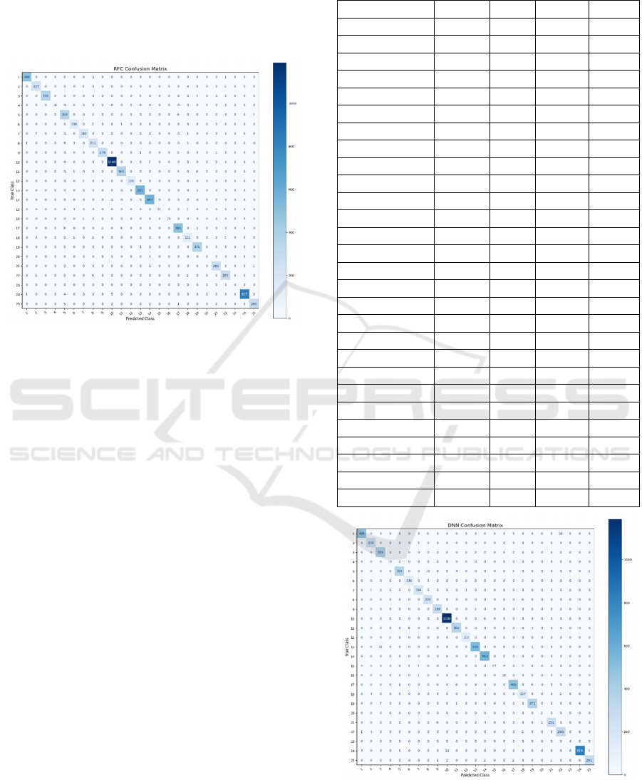
underrepresented classes, indicating occasional

misclassifications. Very small classes again showed

extreme metric values, which may be indicative of

overfitting. The confusion matrix (Fig.7) illustrates

the patterns of misclassification and highlights the

model’s general strengths and limitations.

Figure 7: Confusion matrix of the image data used in the

study using RFC.

3.3 DNN-Based Classification

Outcomes of Remotely Sensed

Multispectral Data

Finally, a Deep Neural Network (DNN) model was

trained and tested to assess the effectiveness of a deep

learning-based approach. The multispectral remote

sensing dataset was divided into training (80%) and

testing (20%) subsets. Evaluation metrics for each

class are presented in Table 4, while the confusion

matrix is provided in Figure 8. These results

demonstrate the DNN model’s capability to capture

complex patterns in the multispectral data and serve

as a benchmark for comparing machine learning and

deep learning approaches.

The DNN model achieved an overall accuracy of

97%, with weighted average precision, recall, and F1-

score also at 97%, indicating a strong and balanced

performance across the dataset. While the model

performed well for most classes, some

underrepresented classes exhibited lower recall

values, reflecting occasional misclassifications. Very

small classes showed extreme metric values in some

cases, which may indicate overfitting rather than

genuine predictive performance. The confusion

matrix (Figure 8) illustrates the distribution of

misclassifications and highlights the general

strengths and limitations of the model.

Table 4: Classification report for the DNN model applied to

the image data used in the study.

Class Precision Recall F1-score Support

1 0.99 0.95 0.97 492

2 0.96 0.99 0.97 235

3 0.90 1.00 0.95 359

4 0.86 1.00 0.93 19

5 0.99 0.94 0.96 378

6 0.95 0.98 0.96 133

7 0.94 0.99 0.97 188

8 0.91 0.97 0.94 226

9 0.95 0.99 0.97 283

10 0.98 0.99 0.99 1194

11 0.97 0.98 0.97 371

12 0.99 0.93 0.93 122

13 0.98 0.94 0.96 562

14 0.98 0.99 0.99 568

15 1.00 0.75 0.86 36

16 0.82 0.95 0.88 19

17 0.99 0.94 0.96 512

18 0.91 0.96 0.94 143

19 0.98 0.98 0.86 379

20 0.67 1.00 0.98 2

21 1.00 0.96 0.98 262

22 0.94 0.98 0.96 297

23 1.00 1.00 1.00 4

24 1.00 0.98 0.99 837

25 0.99 0.97 0.98 299

Accurac

0.97 7920

Macro Av

0.95 0.96 0.95 7920

Wei

hted Av

0.97 0.97 0.97 7920

Figure 8: Confusion matrix of the image data used in the

study using DNN.

Data Complexity-Oriented Classiﬁcation of Multispectral Remote Sensing Imagery via Machine and Deep Learning Approaches

263

4 DISCUSSION AND

CONCLUSION

Classification reports are presented in Tables 2, 3, and

4, respectively, and confusion matrices are presented

in Figs. 6, 7, and 8, respectively, obtained from the

three classification methods: SVM, RFC, and DNN.

Accuracy, precision, recall, and f1 score are

calculated from the confusion matrix results.

The overall accuracies of the SVM, RFC, and

DNN are 0.96, 0.99, and 0.95 in Table 2, Table 3, and

Table 4, respectively. As explained in Section 2, the

best classification accuracy result calculated from the

DNNs is 0.95 due to data complexity. Based on the

results in the precision and/or recall columns, the f1-

score columns of SVM and RFC cannot distinguish

or classify some classes, as can be seen in Tables 2

and 3. However, based on the results in the precision

and recall columns, the f1-score column of DNN can

distinguish or classify all classes, as can be seen in

Table 4. Due to the greater number of processing

layer steps, the processing time is the longest for

DNN.

The findings of this study indicate that when the

data complexity is low, classification can be

effectively performed using machine learning

techniques, whereas high data complexity may

require the utilization of deep learning approaches.

REFERENCES

Thyagharajan, K. K., & Vignesh, T. (2019). Soft computing

techniques for land use and land cover monitoring with

multispectral remote sensing images: A

review. Archives of Computational Methods in

Engineering, 26(2), 275-301.

Modica, G., De Luca, G., Messina, G., & Praticò, S. (2021).

Comparison and assessment of different object-based

classifications using machine learning algorithms and

UAVs multispectral imagery: A case study in a citrus

orchard and an onion crop. European Journal of

Remote Sensing, 54(1), 431-460.

Sishodia, R. P., Ray, R. L., & Singh, S. K. (2020).

Applications of remote sensing in precision agriculture:

A review. Remote sensing, 12(19), 3136.

Guanter, L., Rossini, M., Colombo, R., Meroni, M.,

Frankenberg, C., Lee, J. E., & Joiner, J. (2013). Using

field spectroscopy to assess the potential of statistical

approaches for the retrieval of sun-induced chlorophyll

fluorescence from ground and space. Remote Sensing of

Environment, 133, 52-61.

Thenkabail, P. S., Lyon, J. G., & Huete, A. (2016).

Hyperspectral remote sensing of agriculture and

vegetation. Remote Sensing of Environment, 185, 1–17.

https://doi.org/10.1016/j.rse.2016.01.005

Erol, H., & Akdeniz, F. (2005). A per-field classification

method based on mixture distribution models and an

application to Landsat Thematic Mapper data.

International Journal of Remote Sensing, 26(6), 1229–

1244. https://doi.org/10.1080/01431160512331326800

Sehgal, S. (2012). Remotely sensed LANDSAT image

classification using neural network approaches.

International Journal of Engineering Research and

Applications, 2(5), 43–46.

Calış, N., & Erol, H. (2012). A new per-field classification

method using mixture discriminant analysis. Journal of

Applied Statistics, 39(10), 2129–2140.

https://doi.org/10.1080/02664763.2012.702263

Crnojević, V., Lugonja, P., Brkljač, B., & Brunet, B.

(2014). Classification of small agricultural fields using

combined Landsat-8 and RapidEye imagery: Case

study of northern Serbia. Journal of Applied Remote

Sensing, 8(1), 083512.

https://doi.org/10.1117/1.JRS.8.083512

Gogebakan, M., & Erol, H. (2018). A new semi-supervised

classification method based on mixture model

clustering for classification of multispectral data.

Journal of the Indian Society of Remote Sensing, 46(8),

1323–1331. https://doi.org/10.1007/s12524-018-0808-

Sicre, C. M., Fieuzal, R., & Baup, F. (2020). Contribution

of multispectral (optical and radar) satellite images to

the classification of agricultural surfaces. International

Journal of Applied Earth Observation and

Geoinformation, 84, 101972.

https://doi.org/10.1016/j.jag.2019.101972

Dash, P., Sanders, S. L., Parajuli, P., & Ouyang, Y. (2023).

Improving the accuracy of land use and land cover

classification of Landsat data in an agricultural

watershed.

Remote Sensing, 15(16), 4020.

https://doi.org/10.3390/rs15164020

Kadavi, P. R., & Lee, C. W. (2018). Land cover

classification analysis of volcanic island in Aleutian

Arc using an artificial neural network (ANN) and a

support vector machine (SVM) from Landsat imagery.

Geosciences Journal, 22(5), 653–665.

https://doi.org/10.1007/s12303-018-0023-2

Singh, M. P., Gayathri, V., & Chaudhuri, D. (2022). A

simple data preprocessing and postprocessing

techniques for SVM classifier of remote sensing

multispectral image classification. IEEE Journal of

Selected Topics in Applied Earth Observations and

Remote Sensing, 15, 1–10.

https://doi.org/10.1109/JSTARS.2022.3201273

Pal, M. (2005). Random forest classifier for remote sensing

classification. International Journal of Remote Sensing,

26(1), 217–222.

https://doi.org/10.1080/01431160412331269698

Zhang, H., Li, Q., Liu, J., Shang, J., Du, X., McNairn, H.,

Champagne, C., Dong, T., & Liu, M. (2017). Image

classification using RapidEye data: Integration of

spectral and textual features in a random forest

classifier. IEEE Journal of Selected Topics in Applied

Earth Observations and Remote Sensing, 10(12), 1–10.

https://doi.org/10.1109/JSTARS.2017.2774807

ICEEECS 2025 - International Conference on Advances in Electrical, Electronics, Energy, and Computer Sciences

264

Singh, G., Vyas, N., Dahiya, N., Singh, S., Bhati, N., Sood,

V., & Gupta, D. K. (2025). A novel pixel-based deep

neural network in posterior probability space for the

detection of agriculture changes using remote sensing

data. Remote Sensing Applications: Society and

Environment, 38, 101591.

https://doi.org/10.1016/j.rsase.2025.101591

Erol, H., & Erol, R. (2018). Determining big data

complexity using hierarchical structure of groups and

clusters in decision tree. In Proceedings of the 3rd

International Conference on Computer Science and

Engineering (UBMK’18) (pp. 594–597). IEEE.

https://doi.org/10.1109/UBMK.2018.8566398

Vapnik, V. (2013). The nature of statistical learning theory.

Springer Science & Business Media.

Kadavi, P. R., & Lee, C. W. (2018). Land cover

classification analysis of volcanic island in Aleutian

Arc using an artificial neural network (ANN) and a

support vector machine (SVM) from Landsat imagery.

Geosciences Journal, 22, 653–665.

https://doi.org/10.1007/s12303-018-0023-2

Breiman, L. (1999). Random forests—random features

(Tech. Rep. No. 567). University of California,

Berkeley, Department of Statistics.

Schmidhuber, J. (2014). Deep learning in neural networks:

An overview. Neural Networks, 61, 85–117.

https://doi.org/10.1016/j.neunet.2014.09.003

Dalianis, H. (2018). Evaluation metrics and evaluation. In

Clinical text mining: Secondary use of electronic

patient records (pp. 45–53). Springer.

Google Research. (2025). Google Colab.

https://colab.research.google.com/

Data Complexity-Oriented Classiﬁcation of Multispectral Remote Sensing Imagery via Machine and Deep Learning Approaches

265