Future Vibration Estimation Using LSTM for Condition-Based

Maintenance of Aircraft Systems

Hüseyin Şahin

and Ömer Faruk Göktaş

Vocational School of Technical Science, Ankara Yildirim Beyazit University, Ankara, Turkey

Keywords: Deep Learning, Aircraft System, Vibration Prediction, Predictive Maintenance, Condition-Based

Maintenance.

Abstract: This study presents a deep learning-based approach for enhancing Condition-Based Maintenance (CBM)

strategies in aircraft systems by utilizing Long Short-Term Memory (LSTM) networks to forecast future

vibration trends. Using high-resolution time-series data from the NASA IMS Bearing Dataset, the proposed

LSTM model successfully captures complex temporal dependencies that characterize degradation behaviour

in aircraft components. Experimental results demonstrate that the model achieves high prediction accuracy

with a low Mean Absolute Error (MAE) of 0.0010, enabling timely detection of incipient faults and

minimizing unnecessary maintenance interventions. Compared to traditional models, LSTM networks offer

high performance in learning nonlinear patterns and maintaining predictive reliability under varying

operational conditions. The integration of LSTM-based forecasting into CBM frameworks supports proactive

maintenance planning, reduces lifecycle costs, and increases aircraft safety. This study contributes to the

literature by validating the practical implementation of LSTM in real-world aerospace maintenance

workflows, offering a scalable and intelligent solution for predictive maintenance in both civil and military

aviation contexts.

1 INTRODUCTION

In modern aircraft systems, reliability and safety are

important. Conventional maintenance strategies such

as corrective or time-based maintenance often result

in either excessive downtime or the risk of undetected

failures. In contrast, Condition-Based Maintenance

(CBM) offers a proactive and data-driven solution

that enables timely interventions based on the actual

health status of aircraft components (Choi et al.,

2016).

CBM constitute a paradigm shift in aircraft

engineering, promising significant enhancements in

the efficiency and safety of aircraft systems. Unlike

traditional maintenance strategies that rely on time-

based schedules or reactive responses to mechanical

failures. CBM uses real-time data to assess the

ongoing health of aircraft components. This proactive

approach is facilitated by the integration of advanced

sensors and monitoring technologies that gather

crucial information such as vibration patterns,

https://orcid.org/0000-0003-0464-2644

https://orcid.org/0000-0002-2021-4052

temperature fluctuations or pressure levels

(Kabashkin & Perekrestov, 2024). By analysing these

data, CBM enables the timely identification of

potential failures, allowing maintenance actions to be

precisely aligned with the actual condition of the

components. This not only prevents unnecessary

maintenance interventions but also minimizes the risk

of unexpected downtimes or catastrophic failures.

Thereby improve the reliability and availability of

aircraft systems. In the context of aircraft industry,

where operational efficiency and safety are important,

CBM emerges as an indispensable tool for modern

aircraft maintenance strategies (Verhagen et al.,

2023).

A key advantage of CBM in aircraft is integration

with health monitoring systems and machine learning

algorithms, which allow for fault prediction and

anomaly detection. These capabilities not only

increase operational efficiency but also improve

flight safety by preventing failures. For example,

research by Ozkat et al. showed that deep learning

¸Sahin, H. and Gökta¸s, Ö. F.

Future Vibration Estimation Using LSTM for Condition-Based Maintenance of Aircraft Systems.

DOI: 10.5220/0014299800004848

Paper published under CC license (CC BY-NC-ND 4.0)

In Proceedings of the 2nd International Conference on Advances in Electrical, Electronics, Energy, and Computer Sciences (ICEEECS 2025), pages 169-175

ISBN: 978-989-758-783-2

169

models applied to vibration sensor data on a real-time

UAV can predict when it will fail and provide a

critical window for preventive action (Ozkat et al.,

2023).

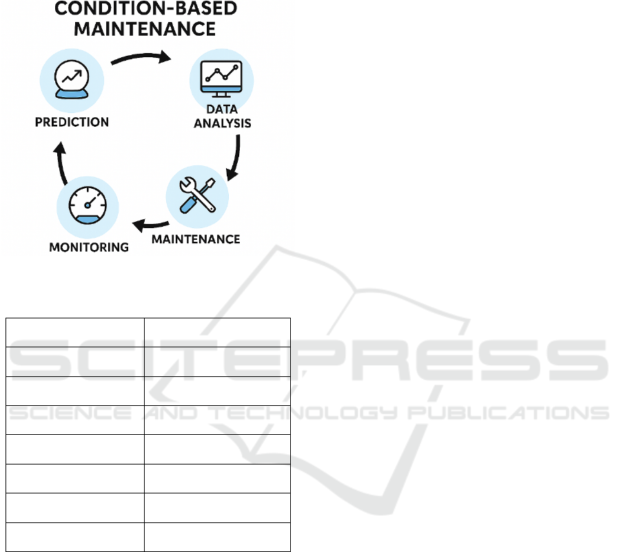
Figure 1: Schematic representation of CBM process.

Table 1: Advantages and disadvantages of RUL forecasting.

Benefits of RUL

Forecasting

Challenges in RUL

Forecasting

Proactive maintenance

lannin

Uncertainty and forecast

accurac

Prevention of

unex

ected failures

Complex system

namics

Optimizing maintenance

costs

Insufficient historical data

Increasing equipment

availabilit

Impact of environmental

factors

Improving spare parts

inventor

mana

ement

Presence of multiple

failure modes

Increasing operational

securit

Sensor noise and errors

Efficient use of

resources

Computational

complexit

Moreover, CBM has been adopted in both civil

and military aircraft applications, including programs

such as Health and Usage Monitoring Systems

(HUMS) used in helicopters and Integrated Vehicle

Health Management (IVHM) systems in fixed-wing

aircraft(Hünemohr et al., 2022; Scott et al., 2022).

The use of CBM has led to cost savings and

maintenance performance, as noted by the U.S.

Department of Defense's CBM+ initiative

(Department of Defense, 2024).

In summary, CBM is an innovative approach in

aircraft maintenance planning. Its capacity to

synchronise maintenance operations with the

prevailing conditions of the system, thereby

minimising the necessity for unscheduled

maintenance interventions, and its ability to facilitate

the implementation of predictive analytics, renders it

an indispensable instrument for the future generation

of aircraft safety and sustainability. The primary aim

of this study is to evaluate the effectiveness of CBM

applications in reducing maintenance costs and

enhancing operational efficiency in aircraft systems.

The necessity for such improvements stems from the

limitations of traditional maintenance approaches. The

utilisation of CBM allows for the synchronisation of

maintenance operations with the true condition of

aircraft components (Cusati et al., 2021). This

approach has the potential to synchronise maintenance

practices with performance requirements, thereby

reducing the overall cost of aircraft operations over

their lifecycle. Furthermore, the use of CBM systems

has been found to enhance the operational reliability

and safety of military and civilian aircraft systems.

(Ernest Yat-Kwan Wong et al., 2006). The study's aim

is to provide empirical evidence and insights into the

cost-effectiveness and operational advantages of

integrating CBM methodologies into current aircraft

maintenance models.

The methodology deployed in this study uses Long

Short-Term Memory (LSTM) models to analyse

vibration data for CBM systems. The study focuses on

the importance of predictive maintenance in aircraft,

and on the capabilities of LSTM in processing time-

series data, which is crucial for understanding and

predicting the future states of aircraft components.

LSTM networks are especially appropriate for

modelling sequential data with long-range temporal

correlations (Malhotra et al., 2016). The integration of

LSTM models in the analysis is a key aspect of the

approach, with the objective being to achieve

enhanced prediction accuracy (Peringal et al., 2024).

The potential real-world implications of research

on CBM within the aircraft discipline are of

considerable importance. The adoption of a predictive

and data-driven approach, as opposed to the traditional

reactive maintenance strategy, enables CBM to

implement interventions prior to the occurrence of

failures. This proactive strategy has been shown to

have a significant impact on maintenance costs, with

a consequent reduction in aircraft downtime and

enhancement of system reliability. Through the

integration of CBM strategies, maintenance activities

in aircraft systems can be aligned more closely with

actual equipment condition, allowing for optimized

scheduling, reduced downtime and increased overall

mission reliability. Consequently, CBM applications

offer considerable economic and operational

advantages, further encouraging the thorough

ICEEECS 2025 - International Conference on Advances in Electrical, Electronics, Energy, and Computer Sciences

170

evaluation and advancement of predictive techniques,

such as the LSTM models investigated in this study,

to enhance the efficiency of these systems in real-

world operational applications.

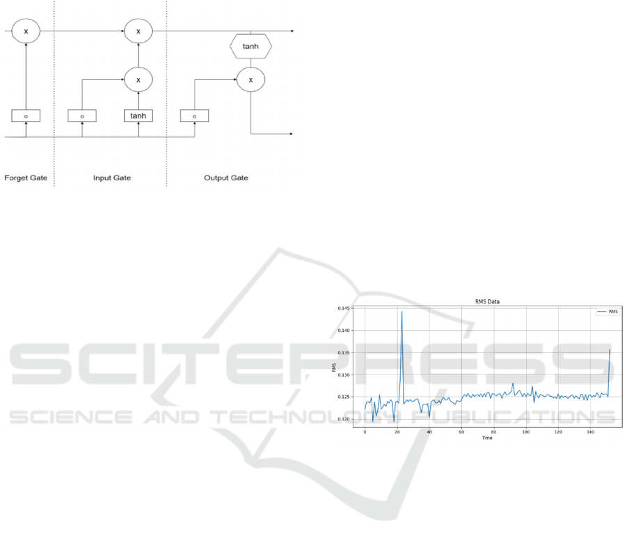
Figure 2 LTSM Neural Network Architecture.

The potential real-world implications of research

on CBM within the aircraft discipline are of

considerable importance. The adoption of a predictive

and data-driven approach, as opposed to the

traditional reactive maintenance strategy, enables

CBM to implement interventions prior to the

occurrence of failures. This proactive strategy has

been shown to have a significant impact on

maintenance costs, with a consequent reduction in

aircraft downtime and enhancement of system

reliability. Through the integration of CBM

strategies, maintenance activities in aircraft systems

can be aligned more closely with actual equipment

condition, allowing for optimized scheduling,

reduced downtime and increased overall mission

reliability. Consequently, CBM applications offer

considerable economic and operational advantages,

further encouraging the thorough evaluation and

advancement of predictive techniques, such as the

LSTM models investigated in this study, to enhance

the efficiency of these systems in real-world

operational applications.

2 METHODOLOGY

The vibration data used in this study were obtained

from the NASA IMS Bearing Dataset, a recognised

standard in the field of condition monitoring research

(J. Lee et al., 2007). This dataset consists of

continuous vibration measurements which reflect the

life cycles of bearings under applied loads. These

measurements are effective in simulating mechanical

degradation in real-world conditions. The high-

resolution, time-series data is essential for predictive

maintenance modelling. The dataset provides a robust

foundation for the application of LSTM networks in

estimating future vibration trends. The selection of

this dataset, which includes critical failure modes,

ensures that the research methodology is well-suited

to address challenges in the implementation of CBM

in aircraft systems.

The vibration data used in this study were

obtained from a bearing test rig developed by the NSF

I/UCRC Intelligent Maintenance Systems Center in

the United States. The test rig consists of four

Rexnord ZA-2115 double row ball bearings

connected to a shaft rotating at a constant speed of

2000 RPM. A radial load of 6000 pounds (~26700 N)

was applied to the shaft and all bearings were

operated with a forced lubrication system. Vibration

data was collected by means of high precision

piezoelectric ICP accelerometers type PCB 353B33

mounted on the bearing housings. In the first data set,

a total of two axes of data were collected for each

bearing in the x and y axes, while in the other sets

only single axis measurements were made(Qiu et al.,

2006).

Figure 3: RMS Vibration Data for Bearing.

The preprocessing of vibration data is a critical

step in preparing it for LSTM model training, and it

is essential to ensure the quality and integrity of the

input. Initially, the raw vibration signals from the

NASA IMS Bearing Dataset are subjected to Min-

Max normalization. This technique is employed to

scale the data range between 0 and 1, thus helping to

minimise the effects of varying scales and

magnitudes, consequently enabling improved

convergence during the training phase. This approach

is crucial in ensuring that each feature contributes

equally to the gradient descent optimisation process,

thus preventing discrepancies that may arise from

differing units and ranges. Following this, the

normalized data is processed by generating window-

based sequences, a step that configures the time-

series data into a structured format suitable for LSTM

input. Each sequence is characterised by a

predetermined number of time steps, which are

represented by a multidimensional array, thereby

Future Vibration Estimation Using LSTM for Condition-Based Maintenance of Aircraft Systems

171

conforming to the LSTM's requirement for

continuous temporal data inputs. The subsequent

phase involves the extraction of features, with the aim

of reducing the dimensionality of the data set and

thereby extracting meaningful information. This

process employs Root Mean Square (RMS) metrics

as a means of quantifying the variability of the data.

The RMS value, calculated over each time window,

represents an aggregate of vibration magnitude,

serving as a key indicator of bearing condition and

mechanical health. By transforming the data into this

comprehensive format, the preprocessing pipeline

equips the LSTM model with precise and statistically

comprehensive inputs, enhancing its ability to predict

future vibration trends accurately.

The LSTM neural network was implemented to

model time-series vibration data, thanks to its ability

to identify long-range dependencies. The LSTM

architecture comprises multiple layers that are

designed to handle the sequence prediction tasks that

are particular to the dataset. At its core, the network

comprises an input layer, followed by a series of

(LSTM) layers. These layers incorporate cells that are

structured to retain information across time steps

through gates, namely input, forget and output gates.

This enables the network to effectively retain memory

and learn sequences. The network uses a

configuration of hidden layers comprising LSTM

blocks stacked on top of each other. Each block

processes a specific aspect of the temporal data (Al-

Selwi et al., 2024). LSTM networks are an enhanced

form of recurrent neural networks (RNNs). The

hidden layer of an LSTM network has a gated unit,

also known as a gated cell. The LSTM consists of four

interconnected layers that produce the cell's output

and cell state. These two layers are then transferred to

the next hidden layer. LSTMs consist of three logistic

sigmoid gates and one tanh layer.

The forget gate is crucial to an LSTM network

because it discards information that is irrelevant for

the current prediction context. When the gate outputs

a value close to zero, the corresponding content is

effectively eliminated from the cell state. Conversely,

an output near one ensures that the information is

retained for subsequent time steps. The input gate

enables new data, relevant information to be

integrated into the cell state. This selective update is

derived from processed input data and modulated by

a learnt weight structure. Finally, the output gate

determines which parts of the current cell state are

propagated to the next layer or output. This shapes the

model's final prediction at that time step.

The LSTM models were trained and validated

using Python as the primary programming

environment and TensorFlow and Keras as the

frameworks for creating and refining the neural

network architecture. The LSTM model was designed

using a sequential layer setup to take full advantage

of Keras's high-level capabilities and streamline the

implementation process. In order to prepare the

network for rigorous testing, the model underwent

several iterations in order to calibrate

hyperparameters such as the number of hidden units,

learning rate, and batch size. The Python libraries

NumPy and Pandas were instrumental in the

management of data operations and the facilitation of

the execution of the training pipeline. Regular

checkpoints were conducted throughout the iterative

process to capture the model's state, guaranteeing a

robust recovery procedure if necessary. The

evaluation of the trained LSTM models was

conducted within the same framework, using a test set

that was separated at the outset of the data processing

workflow to ensure the maintenance of unbiased

evaluation metrics. The implementation of these

methodologies ensured the establishment of a reliable

predictive model capable of estimating future

vibration trends with a high degree of accuracy.

The visualisation of results and the evaluation of

prediction accuracy are critical components of the

research methodology, facilitating in-depth analysis

of the LSTM model's performance. For the purposes

of this study, the Python library Matplotlib was

utilised in order to create comprehensive

visualisations. These tools enabled the creation of

various plots, including line graphs showing

predicted and actual vibration trends over time,

thereby facilitating a clear visual comparison. The

assessment of the model's accuracy was conducted by

utilising standardised metrics, namely the mean

absolute error (MAE) and the root mean square error

(RMSE). These metrics offer quantifiable indicators

of prediction accuracy and are imperative for the

evaluation of the model's validity. The analysis was

enriched with graphical plots, which highlighting the

model's ability to track actual trends and identify

potential inconsistencies. This information forms the

basis for understanding the model's predictive

capacity in real-world aircraft and space CBM

scenarios.

3 RESULTS

The LSTM architecture demonstrated a strong

capability in forecasting future trends in RMS

vibration data, a critical aspect for the effective

implementation of condition-based maintenance in

ICEEECS 2025 - International Conference on Advances in Electrical, Electronics, Energy, and Computer Sciences

172

aircraft systems. The network was able to process

high-frequency signals obtained from the IMS

Bearing Dataset effectively by leveraging its strength

in modelling temporal dependencies. The system's

capacity to monitor and analyse minute yet

substantial variations in RMS values over time allows

for the early identification of degradation indicators,

often preceding the onset of apparent system failures.

This predictive advantage enhances the ability of

maintenance teams to initiate timely interventions,

thereby contributing to improved operational safety

and logistical efficiency in aircraft. Furthermore, the

model enables more strategic maintenance planning

by continuously monitoring vibration behaviour and

providing reliable short-term forecasts. This results in

minimised unnecessary servicing and optimised

resource use and cost-efficiency. The enhanced

performance of the LSTM model is attributable to its

design, which is optimally suited to the analysis of

sequential data. This model is a highly effective

analytical tool for advancing condition-based

maintenance in aircraft applications.

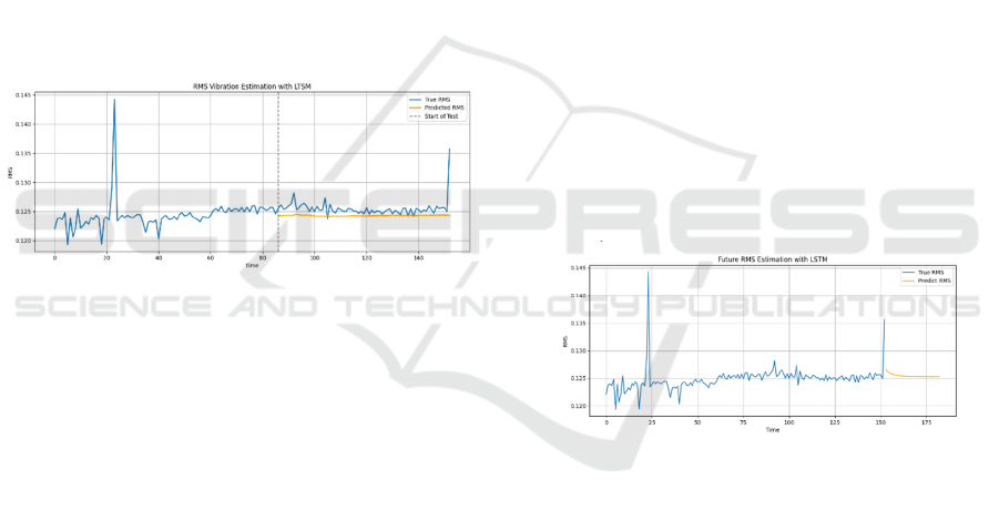
Figure 4: The prediction result used 50% as training data

and 50% as test data

The LSTM model demonstrated a remarkable

capacity to precisely forecast future RMS vibration

trends, a capability that is of paramount importance

for condition-based maintenance of aircraft systems.

The model uses its realistic ability to understand

complex time patterns to create a model of high-

frequency vibration data from the IMS Bearing

Dataset. The model's capacity to forecast alterations

in RMS values over time signifies its ability to discern

subtle yet substantial changes in component

conditions prior to the manifestation of evident

issues. The implementation of this process enables

team members to engage in proactive actions, thereby

facilitating enhanced safety standards and optimising

operational efficiency, a particularly salient

consideration within the domain of aircraft

engineering and maintenance. Maintenance

professionals are able to enhance their planning

processes, avoid unnecessary actions, and achieve

financial and temporal efficiencies by monitoring

RMS trends and making accurate predictions. The

LSTM model's capacity for accurate prediction is

attributable to its design, which is optimally suited to

the analysis of time-based data. This development

indicates that the system is a powerful tool for

improving condition-based maintenance in aircraft

systems.

The predictive performance of the LSTM model

was systematically assessed through a set of widely

recognized evaluation metrics, namely MAE and

RMSE. The model demonstrated a strong predictive

capability, achieving a low MAE of 0.0010, which

indicates high accuracy in estimating future RMSE

vibration patterns in aircraft system components.

Additionally, the RMSE value approaching zero

reinforces this finding by reflecting minimal

divergence between predicted and actual values

across the time series. However, the observed R²

value of -0.6838points to limitations in the model’s

ability to explain variance within the dataset, which

can be attributed to the complex and highly nonlinear

nature of the underlying degradation mechanisms.

This discrepancy suggests that while the model is

effective in short-term trend prediction, it may face

challenges in modelling long-term structural variance

in highly stochastic systems. These results support the

model’s applicability in real-world aircraft

maintenance workflows, where timely and accurate

predictions are essential for ensuring operational

reliability and cost-effectiveness.

Figure 5: The prediction result used 100% as training data.

The strong ability of the LSTM network to model

sequences gives it a clear advantage compared to

traditional predictive models, especially in the field

of condition-based maintenance. LSTM networks are

explicitly designed to learn and preserve long-term

dependencies through a gated memory cell

architecture. This design enables them to dynamically

adjust to evolving data distributions and recognize

intricate vibration patterns that may precede

mechanical failures. The model's robustness in such

contexts is reflected in its consistently low prediction

errors, even under varying operational conditions and

non-uniform degradation rates. The ability of LSTM

models to retain relevant historical information and

update internal representations in response to new

input makes them particularly effective in early

Future Vibration Estimation Using LSTM for Condition-Based Maintenance of Aircraft Systems

173

anomaly detection and maintenance forecasting.

Consequently, their integration into predictive

maintenance pipelines represents a significant leap

forward in aircraft maintenance planning, enabling

data-driven, cost-efficient, and proactive

interventions that improve overall system reliability

and operational safety.

4 DISCUSSION AND

CONCLUSIONS

This study emphasises the pivotal function of LSTM

networks in optimising the execution of CBM

strategies within the aircraft engineering industry.

The proposed model enables high-accuracy

forecasting of future vibration behaviour, thereby

signifying a methodological departure from

conventional maintenance practices. Conventional

maintenance practices are primarily based on fixed

time intervals or reactive repairs following fault

detection. LSTM networks have been demonstrated

to have strong capabilities in modelling nonlinear and

temporally complex datasets, particularly those

derived from the operational behaviour of aircraft

subsystems. This facilitates the early identification of

degradation patterns, thereby enabling predictive

interventions to be implemented before faults evolve

into critical failures. Such foresight supports

maintenance strategies that are both targeted and

timely, significantly reducing unplanned

maintenance and improving the operational safety

and reliability of aircraft in both the civil and defence

industries. The findings of this research affirm that

the integration of LSTM models into CBM

architectures provides a data-driven and adaptive

maintenance paradigm, whereby servicing actions are

aligned with the real-time health status of system

components. This enhanced predictive capability has

been demonstrated to contribute to substantial cost

savings by reducing the need for maintenance and

optimising the efficiency of resource allocation

within aircraft operations.

The present study aims to contribute to the

literature in the field of CBM by integrating LSTM

models and demonstrating the advanced capabilities

of the LSTM architecture compared to traditional

maintenance methods in the aircraft industry. Despite

the limitations of classical regression algorithms and

fundamental artificial neural network structures in

capturing long-term relationships in time series,

LSTM models have demonstrated notable efficacy in

learning and maintaining such intricate temporal

patterns. This feature facilitates more precise

predictions of future vibration trends and has the

potential to extend the lifespan of critical aircraft

components by reducing unnecessary maintenance

interventions. Analyses have demonstrated that

LSTM models achieve lower MAE and RMSE

values, indicating that they enhance the accuracy and

reliability of CBM applications. This has been shown

to result in enhanced system reliability, reduced

unexpected failures and decreased maintenance costs

in operational results. In conclusion, the integration

of LSTM architecture into aircraft maintenance

strategies is not only compatible with artificial

intelligence-based predictive maintenance

approaches, but also offers concrete practical gains

for the maintenance optimisation of aircraft systems.

This makes LSTM models optimal for the

implementation of preventive, economical, and

safety-focused maintenance strategies in

contemporary aircraft.

This research makes a significant contribution to

the academic literature by effectively bridging

theoretical principles with real-world implementation

practices, thereby advancing the comprehension and

applicability of advanced CBM strategies in the field

of aircraft engineering. The study demonstrates that

the deployment of LSTM networks enhances

predictive accuracy, particularly in the context of

forecasting future vibration behaviours. In contrast to

traditional statistical models, the proposed LSTM-

based framework provides a scalable and practical

foundation for real-time CBM integration. The LSTM

model has been developed to learn from complex

temporal sequences, thereby offering a data-driven

mechanism to anticipate component-level

degradation. This, in turn, has the effect of

minimising redundant interventions and improving

overall system availability and reliability. These

findings reflect a paradigm shift from conventional

predictive analytics to intelligent maintenance

strategies, enabling more informed, timely and cost-

effective decision-making processes. Consequently,

this study addresses a critical research gap by

providing empirical validation of LSTM's potential to

transform CBM methodologies and establishes the

foundation for future research into AI-enhanced

maintenance planning in aircraft environments.

REFERENCES

Al-Selwi, S. M., Hassan, M. F., Abdulkadir, S. J., Muneer,

A., Sumiea, E. H., Alqushaibi, A., & Ragab, M. G.

(2024). RNN-LSTM: From applications to modeling

ICEEECS 2025 - International Conference on Advances in Electrical, Electronics, Energy, and Computer Sciences

174

techniques and beyond—Systematic review. Journal of

King Saud University - Computer and Information

Sciences, 36(5), 102068.

https://doi.org/10.1016/J.JKSUCI.2024.102068

Choi, J. H., Kim, N. H., & Kogiso, N. (2016). Reliability

for aerospace systems: Methods and applications.

Advances in Mechanical Engineering, 8(11), 1.

https://doi.org/10.1177/1687814016677092;PAGE:ST

RING:ARTICLE/CHAPTER

Cusati, V., Corcione, S., & Memmolo, V. (2021). Impact of

Structural Health Monitoring on Aircraft Operating

Costs by Multidisciplinary Analysis. Sensors (Basel,

Switzerland), 21(20), 6938.

https://doi.org/10.3390/S21206938

Department of Defense. (2024). Condition-Based

Maintenance Plus Guidebook.

https://www.acq.osd.mil/log/MR/cbm+.html

Ernest Yat-Kwan Wong, Stephen E. Gauther, & Simon R.

Goerger. (2006). Condition-Based Maintenance

(CBM): A Working Partnership between Government,

Industry, and Academia.

https://www.researchgate.net/publication/235093552_

Condition-

Based_Maintenance_CBM_A_Working_Partnership_

between_Government_Industry_and_Academia

Hünemohr, D., Litzba, J., & Rahimi, F. (2022). Usage

Monitoring of Helicopter Gearboxes with ADS-B

Flight Data. Aerospace 2022, Vol. 9, Page 647, 9(11),

647. https://doi.org/10.3390/AEROSPACE9110647

J. Lee, H. Qiu, G. Yu, J. Lin, & Rexnord Technical

Services. (2007). IMS, University of Cincinnati

“Bearing Data Set.” https://data.phmsociety.org/nasa/

Kabashkin, I., & Perekrestov, V. (2024). Ecosystem of

Aviation Maintenance: Transition from Aircraft Health

Monitoring to Health Management Based on IoT and

AI Synergy. Applied Sciences 2024, Vol. 14, Page

4394, 14(11), 4394.

https://doi.org/10.3390/APP14114394

Matias, O., Renna, P., Ali, A., Abdelhadi, A., & Linton, A.

L. (2022). Condition-Based Monitoring and

Maintenance: State of the Art Review. Applied Sciences

2022, Vol. 12, Page 688, 12(2), 688.

https://doi.org/10.3390/APP12020688

Ozkat, E. C., Bektas, O., Nielsen, M. J., & la Cour-Harbo,

A. (2023). A data-driven predictive maintenance model

to estimate RUL in a multi-rotor UAS. International

Journal of Micro Air Vehicles, 15.

https://doi.org/10.1177/17568293221150171/ASSET/

19A20BAC-2FBF-4C54-B27B-

555A8CBD2386/ASSETS/IMAGES/LARGE/10.1177

_17568293221150171-FIG13.JPG

Qiu, H., Lee, J., Lin, J., & Yu, G. (2006). Wavelet filter-

based weak signature detection method and its

application on rolling element bearing prognostics.

Journal of Sound and Vibration, 289

(4–5), 1066–1090.

https://doi.org/10.1016/J.JSV.2005.03.007

Quatrini, E., Costantino, F., Di Gravio, G., & Patriarca, R.

(2020). Condition-Based Maintenance—An Extensive

Literature Review. Machines 2020, Vol. 8, Page 31,

8(2), 31. https://doi.org/10.3390/MACHINES8020031

Scott, M. J., Verhagen, W. J. C., Bieber, M. T., &

Marzocca, P. (2022). A Systematic Literature Review

of Predictive Maintenance for Defence Fixed-Wing

Aircraft Sustainment and Operations. Sensors, 22(18).

https://doi.org/10.3390/S22187070

Verhagen, W. J. C., Santos, B. F., Freeman, F., van Kessel,

P., Zarouchas, D., Loutas, T., Yeun, R. C. K., & Heiets,

I. (2023). Condition-Based Maintenance in Aviation:

Challenges and Opportunities. Aerospace 2023, Vol.

10, Page 762, 10(9), 762.

https://doi.org/10.3390/AEROSPACE10090762

Future Vibration Estimation Using LSTM for Condition-Based Maintenance of Aircraft Systems

175