Differential Kinematics Control Using Circles as Bivectors of Conformal

Geometric Algebra

Julio Zamora-Esquivel

1 a

, Alberto Jaimes Pita

1 b

, Edgar Macias-Garcia

1 c

, Javier Felip-Leon

1 d

David Gonzalez-Aguirre

1 e

and Eduardo Bayro-Corrochano

2 f

Intelligent System Research, Intel Labs, Zapopan, Jalisco, Mexico

Poznan University of Technology, Poznan, Poland

Keywords:

Grasping, Kinematics, Manipulation Planning.

Abstract:

In this paper, we propose a modern mathematical framework to model a robotic arm and compute the dif-

ferential kinematics of its end effector, which is represented as a circle in a three-dimensional space. This

circle is described using a bi-vector within the context of conformal geometric algebra. By utilizing a circle

to characterize the grasping pose on the object and the pose of the end-effector, we develop a differential

kinematics-based control law that guides the end-effector to minimize the error between both circles. The cir-

cle representation offers three degrees of freedom for the center, two degrees for orientation, and one degree

for the radius, allowing us to effectively describe the end-effector pose using a single geometric primitive. Our

approach allows for simultaneous adjustment of both the position and orientation of the end effector.

1 INTRODUCTION

Visually guided grasping is a well-established prob-

lem that has been addressed through various ap-

proaches (Fang et al., 2020), (Wei et al., 2021),

(Fourmy et al., 2023), (Farias et al., 2021). Typically,

it involves developing a control law to adjust the joint

angles of a robotic arm to minimize the error between

the end-effector and the target pose, deﬁned by the

orientation and position, where most of the state-of-

the-art algorithms often tackle this problem by con-

trolling position and orientation independently (Ma

et al., 2020). In contrast, our proposed algorithm em-

ploys a single geometric primitive to simultaneously

describe both the position and orientation of the end-

effector and the target goal. This geometric primitive

is efﬁciently represented as a bivector within the Con-

formal Geometric Algebra (CGA) framework.

As a practical example, we model the kinematics and

differential kinematics of the 7-DoF Franka robot arm

https://orcid.org/0000-0002-0226-0047

https://orcid.org/0009-0009-8339-6605

https://orcid.org/0000-0003-2571-9460

https://orcid.org/0000-0002-2115-4610

https://orcid.org/0000-0002-5032-8261

https://orcid.org/0000-0002-4738-3593

and the Unitree G1 humanoid robot. Our control law,

grounded in the differential kinematics of circles, en-

ables the efﬁcient displacement of both end effectors

to a set of predeﬁned target poses with a cylindrical

geometry p

ob j

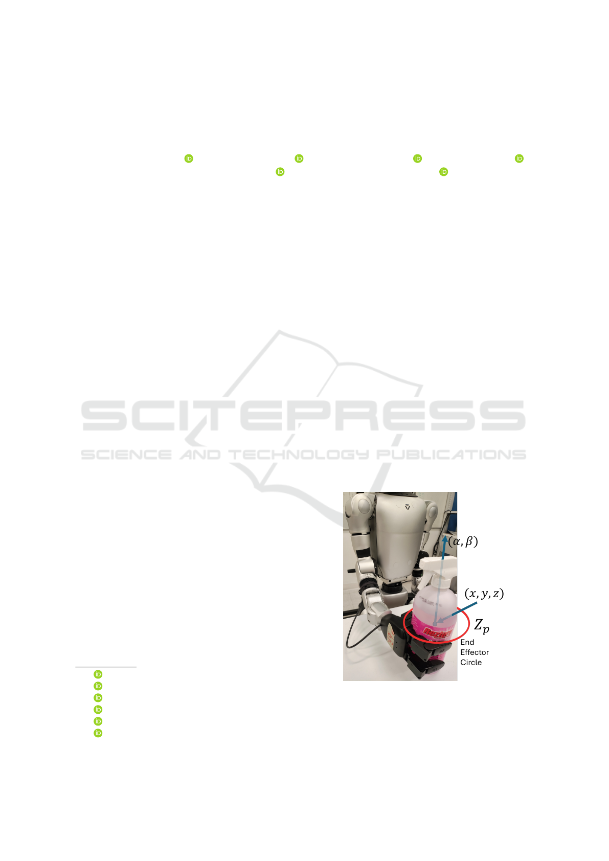
= [x,y, z, α, β] (Figure 1).

Figure 1: End-effector pose of an object described with a

circle Z

∈ G

4,1

in conformal geometric algebra.

Zamora-Esquivel, J., Pita, A. J., Macias-Garcia, E., Felip-Leon, J., Gonzalez-Aguirre, D. and Bayro-Corrochano, E.

Differential Kinematics Control Using Circles as Bivectors of Conformal Geometric Algebra.

DOI: 10.5220/0013945500003982

Paper published under CC license (CC BY-NC-ND 4.0)

In Proceedings of the 22nd International Conference on Informatics in Control, Automation and Robotics (ICINCO 2025) - Volume 2, pages 585-592

ISBN: 978-989-758-770-2; ISSN: 2184-2809

585

The rest of the paper is organized as follows: Sec-

tion 2 provides a brief introduction to Conformal Ge-

ometric Algebra and the representation of circles as

geometric entities. In Section 3, we present our pro-

posed methodology to model and solve the differen-

tial kinematics of end-effectors using circles in Con-

formal Geometric Algebra. Section 4 introduces a

novel approach for applying a control law based on

these techniques, with different practical implemen-

tations on Section 5. Finally, Section 6 discusses the

conclusions and potential directions for future work.

2 CLIFFORD ALGEBRA AND

CONFORMAL GEOMETRY

Geometric algebra (G

4,1

) provides an elegant frame-

work for expressing conformal geometry. To illus-

trate this, we adopt the formulation presented in (Li

et al., 2001) and demonstrate how the Euclidean vec-

tor space (R

) is represented within (R

4,1

). This

space is characterized by an orthonormal vector basis

), with the properties of the Clifford

product detailed in Table 1.

Table 1: Clifford product for blades in Conformal Geomet-

ric Algebra (G

4,1

Basis e

1 e

−e

1 e

−e

1 e

1 E

−E −1

Where e

i j

= e

∧ e

is a bivectorial basis, while e

and e

are the Hamilton basis. A unit Euclidean

pseudo-scalar I

, a pseudo-scalar I

and the bivector

E can be deﬁned by:

: = e

∧ e

, (1)

E : = e

∧ e

= e

, (2)

: = I

∧ E = I

E. (3)

2.1 Geometric Entities

Within this mathematical framework, it is possible to

represent various geometric entities such as points,

lines, planes, circles, and spheres in a 3D space (For

a detailed description, please refer to Bayro (Bayro-

Corrochano, 2018)). This framework enables the rep-

resentation of a point at inﬁnity (e

∞

), and the origin

∞

= e

+ e

, (4)

− e

), (5)

which can be used to deﬁne other geometric entities,

and apply transformations between them. A 3D Eu-

clidean Point (x

∈ G

) can be mapped to a conformal

point (x

∈ G

4,1

) through the transformation:

= x

∞

+ e

. (6)

2.2 Spheres and Planes

The equation of a sphere of radius ρ centered at point

∈ R

can be written as:

− p

)

= ρ

, (7)

since x

· y

= −

− y

)

, we can rewrite the for-

mula above in terms of homogeneous coordinates as:

· p

= −

, (8)

by considering that x

· e

∞

= −1, we can factor the

expression above to:

· (p

−

∞

) = 0. (9)

Which ﬁnally yields the simpliﬁed equation for the

sphere as s = p

−

∞

(note from this equation

that a point is just a sphere with zero radius). Al-

ternatively, the dual of the sphere is represented as

(n + 1)-vectors s

∗

= sI

−1

. The advantage of the dual

form is that the sphere can be directly computed from

four points (in 3D) as:

∗

= x

∧ x

. (10)

If we replace one of these points for the point at inﬁn-

ity we get:

∗

= x

∧ x

∧ e

∞

. (11)

So, as π becomes in the standard form:

π = π

∗

−1

, (12)

π = n + de

∞

, (13)

where n is the normal vector and d represents the

Hesse distance.

2.3 Circles and Lines

A circle z can be regarded as the intersection of two

spheres s

and s

as z = (s

∧ s

). The dual form of

the circle can be expressed by three points:

∗

= x

∧ x

. (14)

COBOTA 2025 - Special Session on Bridging the Gap in COllaborative roBOtics: from Theory to real Applications

586

Similar to the case of planes, lines can be deﬁned by

circles passing through the point at inﬁnity as:

∗

= x

∧ x

∧ e

∞

, (15)

while the standard form of the line (in 3D) can be ex-

pressed by:

L = l + e

∞

(t · l). (16)

The line in the standard form is a bivector, and it has

six parameters (Plucker coordinates), but just four de-

grees of freedom. A full list of entities is described in

Tables 2 and 3.

Table 2: Representation of conformal geometric using the

standard representation.

Entity Representation

Sphere s = p −

∞

Point x

= x

∞

+ e

Line L = π

∧ π

Plane π = n + de

∞

Circle z = s

∧ s

Pair of P. P

= s

∧ s

Table 3: Representation of conformal geometric entities us-

ing the dual representation.

Entity Dual Representation

Sphere s

∗

= x

∧ x

Point x

∗

= s

∧ s

Line L

∗

= x

∧ x

∧ e

∞

Plane π

∗

= x

∧ x

∧ e

∞

Circle z

∗

= x

∧ x

Pair of P. P

∗

= x

∧ x

3 DIFFERENTIAL KINEMATICS

OF CIRCLES

In conformal geometric algebra, the forward kinemat-

ics of the end-effector circle z

∈ R

4,1

is given by

(Hildenbrand et al., 2008):

′

∏

i=1

∏

i=1

n−i+1

. (17)

In this equation motors M are used to represent 3D

rigid transformations as the motor algebra does (E.

and K

ahler, 2000):

M = cos





− sin





L = e

−

, (18)

now we produce an expression for differential kine-

matics through the total differentiation of (17) as fol-

lows:

′

∑

j=1

∂

∏

i=1

∏

i=1

n−i+1

, (19)

where

M is the motor conjugate. Each term of the

sum is the product of two functions in q

, then the

differential yields:

′

∑

j=1

∂

∏

i=1

∏

i= j+1

∏

i=1

n−i+1

∏

i=1

n− j

∏

i=1

n−i+1

∂

∏

i=n− j+1

n−i+1

. (20)

Since M = e

−

, the differential of the motor can be

deﬁned as d(M) = −

MLdq. Thus, we can write the

partial differential of the motor’s product as follows:

∂

∏

i=1

= −

∏

i=1

= −

j−1

∏

i=1

(21)

In a similar approach, the differential of the

M = e

give us d(

M) =

MLdq, and the differential of the

product is:

∂

∏

i=n− j+1

n−i+1

∏

i=n− j+2

n−i+1

(22)

by replacing (21) and (22) in (20) we get:

′

= −

∑

j=1

j−1

∏

i=1

∏

i= j

n− j+1

∏

i=1

n−i+1

−

∏

i= j

n− j+1

∏

i=1

n−i+1

j−1

∏

i=1

j−i

(23)

By deﬁnition the product ”◦” of two bivectors is given

by:

A ◦ B = AB − BA (24)

Using the equation (24) we can simplify (23), since L

and Z

are bivectors then we can rewrite (23) as:

′

∑

j=1

j−1

∏

i=1

∏

i= j

n− j+1

∏

i=1

n−i+1

◦ L

j−1

∏

i=1

j−i

(25)

Differential Kinematics Control Using Circles as Bivectors of Conformal Geometric Algebra

587

The product of i = [1, j − 1] and i = [ j,n] is equal to

the product of i = [1,n]. Also for

M, equation (25)

can be written as:

′

∑

j=1



∏

i=1

∏

i=1

n−i+1



◦



j−1

∏

i=1

j−1

∏

i=1

j−i



(26)

Using the equation of the direct kinematics (17), we

can simplify (26) as:

′

∑

j=1

′

◦

j−1

∏

i=1

j−1

∏

i=1

j−i

. (27)

The equation of forward kinematics of circles also ap-

plies for Lines, in this way we can use (17) to deﬁne

the transformed line L

′

in terms of L as follows:

′

j−1

∏

i=1

j−1

∏

i=1

j−i

. (28)

Finally, by replacing (28) on (27) we get a very com-

pact expression of differential kinematics:

′

∑

j=1



′

◦ L

′



. (29)

4 KINEMATIC CONTROL OF A

ROBOT ARM

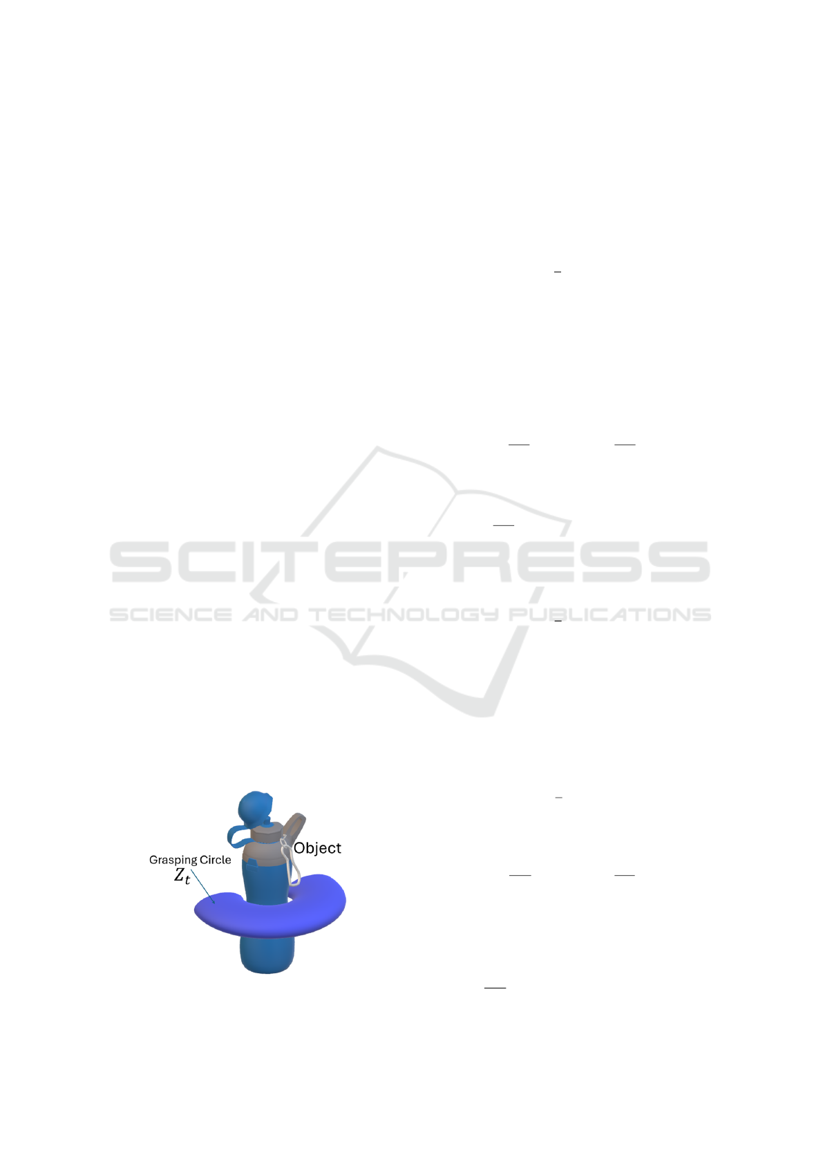
In this section, we ﬁrst deﬁne a control law based on

the orientation of the end effector, followed by a con-

trol law based on its position. These two aspects are

then integrated into a uniﬁed control law that simulta-

neously addresses both position and orientation, uti-

lizing the circle representation to model the pose of

the end-effector and the desired position (Figure 2).

Figure 2: Target circle estimated in the manipulated object.

This kinematic control is formulated as a training rule

for a neural network, utilizing gradient descent to ad-

just the weights, speciﬁcally the joint angles (q). The

primary objective is to adjust the values of q to min-

imize the error, deﬁned as the difference between the

end-effector’s orientation and the target orientation,

as expressed by the following equation:

− Z

)

. (30)

In this context, (Z

) represents the target circle, while

) denotes the circle generated by the gripper as the

end-effector, which describes the pose of the robotic

arm deﬁned by the joints q. This relationship is es-

tablished through the direct kinematics equation, as

given by equation (17). To adjust the joint angles (q)

and minimize the error (E), the partial derivative is

computed as follows:

∂E

∂q

= −(Z

− Z

)

∂Z

∂q

. (31)

In previous sections the differential kinematics was

formulated in terms of the rotation axis L

as:

∂E

∂q

= −(Z

− Z

) ·



◦ L

′



, (32)

now, to create a control law for the position of the end-

effector the error given by the delta in position will be

computed as:

− X

)

, (33)

where P

represents the target position and X

repre-

sents the position of the end effector. Here X

is also

the center of the circle and it can be also replaced by

a sphere S

with the center in the center of the circle:

= Z

/π

, (34)

where π

is the plane of the circle given by π

∗

= Z

∗

∧

∞

. Then the error can be rewritten as:

− S

)

. (35)

The training rule to minimize the error E

by adjust-

ing the joint angles q can be written as:

∂E

∂q

= −(P

− S

)

∂S

∂q

. (36)

According to (Bayro-Corrochano and Zamora-

Esquivel, 2007) the differential kinematics of points

and spheres can be computed using [S

· L

′

]. Then we

can simplify equation (36) as:

∂E

∂q

= −(P

− S

) ·



−1

· L

′



. (37)

COBOTA 2025 - Special Session on Bridging the Gap in COllaborative roBOtics: from Theory to real Applications

588

Thus, we can merge the equations (37) and (32), as

they are vectors and bivectors, respectively. This

merge is achieved through a weighted sum by incor-

porating the learning rates (η

) and (η

), which, in

control terms, represent the gain of the control law.

∂E

∂q

∂E

∂q

= − η

− S

) ·



−1

· L

′



− η

− Z

) ·



◦ L

′



(38)

by reordering the terms:

∂E

∂q

∂E

∂q

= − (η

− S

) + η

− Z

))



(π

−1

+ 1)L

′



(39)

the rule to update the joint angles can be written as:

∆q

=(η

− S

) + η

− Z

))



(π

−1

+ 1)L

′



(40)

where S

, S

are the spheres, and P

is the center of

the sphere S

5 APPLICATIONS

In this section, we implement the differential kine-

matics and control laws described in the previous sec-

tions to model and manipulate the position and orien-

tation of the end-effector for different robots, includ-

ing both single and bi-manual grasping scenarios.

5.1 7DOF Franka Emika Robot Arm

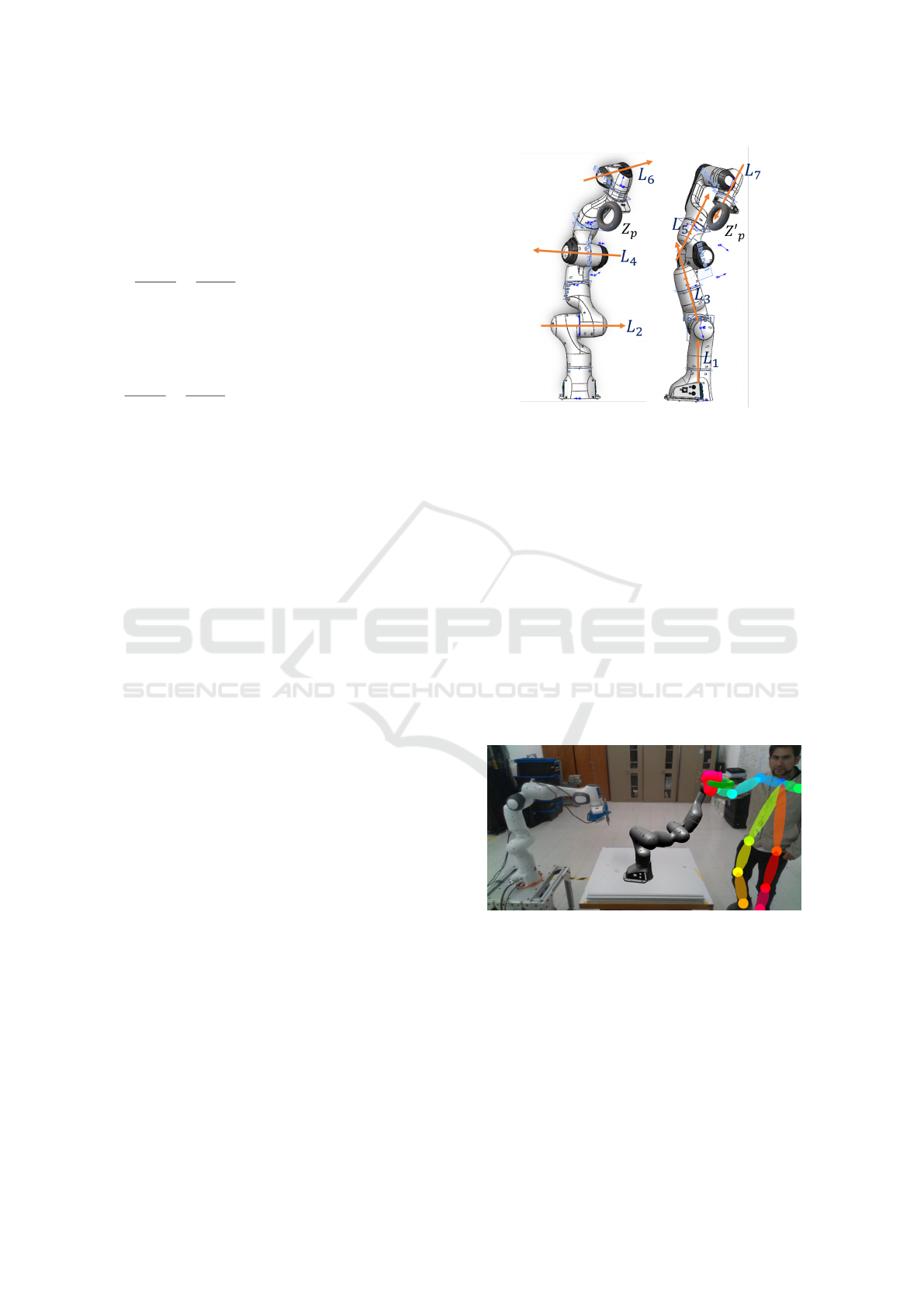
As a ﬁrst experiment, we consider the 7-DoF Franka

Emika robot arm. By employing the equation (17) we

can model the forward kinematics of the end-effector

by employing a set of lines and motors over each joint,

with a circle entity placed on the end-effector (Fig-

ure 3). This formulation allows to describe the posi-

tion and orientation of the end-effector in terms of the

joints position.

To deﬁne the desired position and orientation of

the end effector, we developed a Mixed Reality En-

vironment called Roomersive. This environment has

the capability to display robots and virtual objects in

augmented reality, facilitating real-time interactions

with other users within the same scene (Figure 4).

To enable the interaction between users and the sim-

ulated robot, we implemented a detection system

composed of four Deep Learning Neural Networks

Figure 3: Robot arm Axis represented by lines L

, each one

of those lines is given by a Bivector of conformal geometry.

Models running in parallel, trained for scene un-

derstanding; human pose estimation (based on (Cao

et al., 2017)), face re-identiﬁcation (based on FaceNet

(Schroff et al., 2023)), object recognition (based on

(Wang et al., 2023)), and action recognition (Archana

and Hareesh, 2021). Each model predicts a set of

2D keypoints, which are then converted to 3D and

mapped into the immersive space using data from a

RealSense depth camera. Additionally, this innova-

tive simulator enables the connection of a real robot

with its digital twin within the immersive environ-

ment, by sending the calculated joints to the real robot

and reﬂecting the current real position on the simula-

tor. This feature allows users to manipulate the real

robot by interacting with the virtual object.

Figure 4: Roomersive creates a digital twin of a real robot

within an immersive environment, allowing users to inter-

act with it and transmit information to a real robot located

elsewhere.

To enable the interactions between users and virtual

objects, we employ procedural geometry; This geom-

etry is generated using the Hull and Domain shaders

of DX11/DX12 (Corporation, 2023) on the GPU. Es-

sentially, the depth image is mapped as a texture to the

GPU, and an 8 × 13 array of patches is created, each

with four control points. In the domain shader, each

Differential Kinematics Control Using Circles as Bivectors of Conformal Geometric Algebra

589

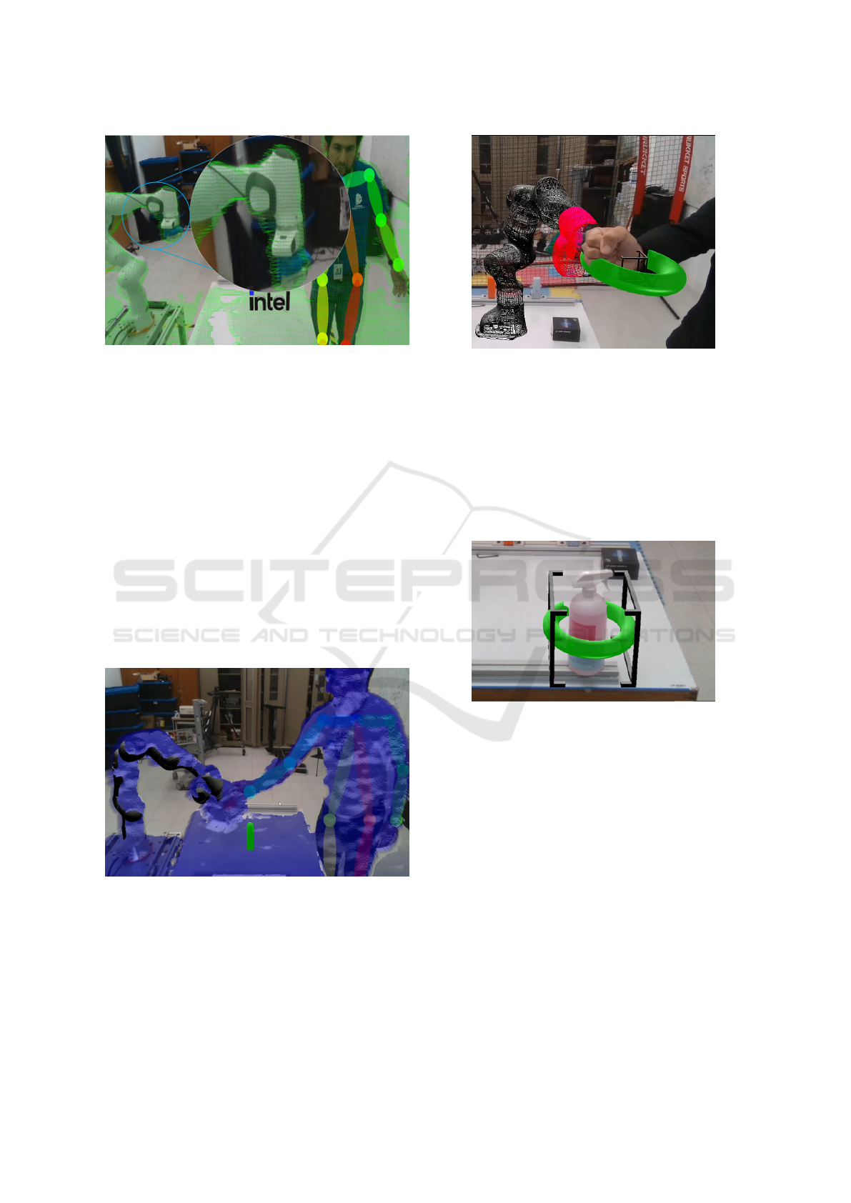
Figure 5: Procedural Geometry created using Depth infor-

mation from Realsense Camera.

patch is tessellated up to 64 × 64, producing 4,096

vertices. For each generated vertex, we sample the

depth information, which is back-propagated to gen-

erate 851,968 triangles per frame (Figure 5).

Rendering integration is achieved by creating a

virtual camera with identical intrinsic parameters and

positioning as the real camera. The image is then

copied to the back buffer, and the procedural geom-

etry is rendered with transparency to facilitate the vi-

sualization (Figure 6). This allows virtual objects to

be occluded by or occlude real objects based on their

positions. The proposed control law is applied in two

scenarios: ﬁrst, to remotely manipulate the robot arm

by grasping and moving the virtual end-effector; and

second, to grasp objects using a grasping circle lo-

cated in the same position than the real objects.

Figure 6: Procedural geometry in blue, used to set the scene

depth on the 3D pipeline.

5.1.1 Immersive Remote Control

In this application we use human pose estimation and

depth information to identify the wrist position in 3D,

and based on the forward kinematics we estimate the

position and orientation of the robot’s end effector

Figure 7: Wrist detection modeled with a circle, used to pull

the virtual robot arm.

described with a circle, when the direct distance be-

tween the wrist circle and the end effector circle is

less than a threshold and the close palm action is de-

tected on the hand, the control law (40) is activated,

this makes the robot follow the hand movement, it is

important to note that we do not require the use of

manual controls that allow the user to manipulate the

objects.

Figure 8: Object detected by our NN in 3D and the circle of

grasping in the Mixed reality space.

5.1.2 Object Grasping

In this scenario, we employ a YOLO-based neural

network to detect objects, using a bottle as an illus-

trative example (Figure 8). Once the object is located

in 3D and isolated within a bounding cube, the tar-

get circle for the object is estimated. This initiates

the control law 40, which guides the robot to grasp

the object by simultaneously aligning its position and

orientation.

5.2 Unitree G1, Humanoid Robot

As an additional experiment, we constructed the Uni-

tree G1 humanoid robot using the same forward kine-

matics procedure applied to the Franka Emika robot

(equation ((17))). We then implemented various in-

COBOTA 2025 - Special Session on Bridging the Gap in COllaborative roBOtics: from Theory to real Applications

590

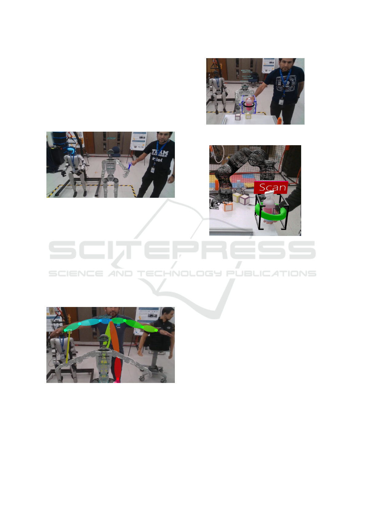
teraction levels in our simulator to manipulate the po-

sition of the joints based on the user’s body pose in-

formation. To facilitate this, we developed models to

identify when the user opens or closes their hands.

Upon detecting that a joint is ”grasped,” we calculate

a pair of circles based on the position and orientation

of the selected joint and the hand. These circles are

then adjusted using our control law to minimize the

error between them (Figure 9).

Figure 9: Interaction level 1: The user can ”grasp” the joint

that he wants to adjust.

Our differential kinematics algorithm can also be ap-

plied to track the human body, adjusting joint angles

to accommodate multiple targets. In this approach,

each joint incrementally adjusts the preceding joints

to achieve the desired position (Figure 10). Addition-

ally, a single target circle can be used to manipulate

multiple end effectors simultaneously, such as in bi-

manual grasping. In the experiment shown in Figure

11, a single target position is deﬁned for both hands

of the robot, enabling it to ”grasp” the object. In this

setup, each joint receives an average of the deltas from

the errors of the two end effectors.

Figure 10: Interaction level 2: Humanoid robot mimicking

human movements using the references of the body pose.

Additionally, other interaction levels can be imple-

mented, for example, by choose the action to do using

the immersive space (Figure 12).

Figure 11: Interaction level 3: A single target desired pose

is deﬁned for both hands.

Figure 12: When the user interacts with an object, a pop-up

virtual menu appears to select the desired action.

5.3 Results Discussion

The aim of this work is not to compete with the state-

of-the-art in terms of speed; rather, it introduces a

modern representation of the end-effector and control

law using circles on the geometric algebra framework,

resulting in equations that are more computationally

efﬁcient. Traditional robot kinematics, typically cal-

culated using matrices, require 64 MAC operations

to concatenate two transformations, whereas confor-

mal geometry rotations require only 16 MAC opera-

tions for concatenation. This control law simultane-

ously addresses both rotation and position, enhancing

efﬁciency. Our immersive reality system eliminates

the need for handheld controllers and virtual reality

glasses, offering a more natural interaction experi-

ence. Figure 13 illustrates the trajectory graph of the

user’s hand in 3D compared to the trajectory of the

end-effector after applying the control law. Human

pose detection, action recognition, and object detec-

tion operate at 60 fps, alongside the procedural gen-

eration and rendering of virtual objects and robots.

Differential Kinematics Control Using Circles as Bivectors of Conformal Geometric Algebra

591

Figure 13: Internal circle components converging after 240

frames (4 seconds).

6 CONCLUSIONS

In this work, the authors aim to demonstrate the fea-

sibility of the new mathematical representation and

control algorithm. By avoiding the use of matrices for

computing kinematics and control, they introduce a

novel formulation based on dual quaternions as bivec-

tors. The authors do not intend to compare perfor-

mance with traditional methods, as matrix operations

are typically accelerated on GPUs, whereas Clifford

algebras are not. Although this method can reduce

MAC operations, the lack of acceleration or paral-

lelization means that results may be comparable in

terms of time, depending on the hardware used. A

separate study focusing on performance, metrics, and

hardware using both approaches will be presented in a

subsequent article. This work is limited to cylindrical

shapes that can be gripped from any position along the

circle. To ensure a unique grip pose, a parabola could

be used instead of a circle, thereby adding additional

degrees of freedom to describe it. This would necessi-

tate the use of Quaternion Geometric Algebra (QGA)

(Zamora-Esquivel, 2014) to calculate the kinematics

and control. We are considering this approach for fu-

ture work.

REFERENCES

Archana, N. and Hareesh, K. (2021). Real-time human ac-

tivity recognition using resnet and 3d convolutional

neural networks. In 2021 2nd International Con-

ference on Advances in Computing, Communication,

Embedded and Secure Systems (ACCESS), pages 173–

177. IEEE.

Bayro-Corrochano, E. (2018). Geometric algebra applica-

tions vol. I: Computer vision, graphics and neurocom-

puting. Springer.

Bayro-Corrochano, E. and Zamora-Esquivel, J. (2007). Dif-

ferential and inverse kinematics of robot devices using

conformal geometric algebra. Robotica, 25(1):43–61.

Cao, Z., Simon, T., Wei, S. E., and Sheikh, Y. (2017). Real-

time multi-person 2d pose estimation using part afﬁn-

ity ﬁelds. In Proceedings of the IEEE conference on

computer vision and pattern recognition, pages 7291–

7299.

Corporation, I. (2023). Directx 12 ultimate on intel® arc™

graphics. Intel. https://www.intel.com/content/www/

us/en/architecture-and-technology/visual-technolog

y/directx-12-ultimate.html.

E., B.-C. and K

ahler, D. (2000). Motor algebra approach

for computing the kinematics of robot manipulators.

Journal of Robotics Systems, 17(9):495–516.

Fang, W., Chao, F., Lin, C. M., Zhou, D., Yang, L.,

Chang, X., and Shang, C. (2020). Visual-guided

robotic object grasping using dual neural network con-

trollers. IEEE Transactions on Industrial Informatics,

17(3):2282–2291.

Farias, C. D., Adjigble, M., Tamadazte, B., Stolkin, R., and

Marturi, N. (2021). Dual quaternion-based visual ser-

voing for grasping moving objects. In 2021 IEEE 17th

International Conference on Automation Science and

Engineering (CASE), pages 151–158. IEEE.

Fourmy, M., Priban, V., Behrens, J. K., Mansard, N., Sivic,

J., and Petrik, V. (2023). Visually guided model pre-

dictive robot control via 6d object pose localization

and tracking. arXiv preprint, arXiv:2311.05344.

Hildenbrand, D., Zamora, J., and Bayro-Corrochano, E.

(2008). Inverse kinematics computation in computer

graphics and robotics using conformal geometric alge-

bra. Advances in applied Clifford algebras, 18:699–

713.

Li, H., Hestenes, D., and Rockwood, A. (2001). General-

ized homogeneous coordinates for computational ge-

ometry. In Somer, G., editor, Geometric Computing

with Clifford Algebras, pages 27–52. Springer-Verlag

Heidelberg.

Ma, Y., Liu, X., Zhang, J., Xu, D., Zhang, D., and Wu,

W. (2020). Robotic grasping and alignment for small-

size components assembly based on visual servoing.

The International Journal of Advanced Manufactur-

ing Technology, 106:4827–4843.

Schroff, F., Kalenichenko, D., and Philbin, J. (2023).

Facenet: A uniﬁed embedding for face recognition

and clustering. In The Computer Vision Foundation.

Retrieved 4 October 2023.

Wang, C. Y., Bochkovskiy, A., and Liao, H. Y. M. (2023).

Yolov7: Trainable bag-of-freebies sets new state-of-

the-art for real-time object detectors. In Proceedings

of the IEEE/CVF conference on computer vision and

pattern recognition, pages 7464–7475.

Wei, H., Pan, S., Ma, G., and Duan, X. (2021). Vision-

guided hand–eye coordination for robotic grasping

and its application in tangram puzzles. AI, 2(2):209–

228.

Zamora-Esquivel, J. (2014). G 6, 3 geometric algebra; de-

scription and implementation. Advances in Applied

Clifford Algebras, 24(2):493–514.

COBOTA 2025 - Special Session on Bridging the Gap in COllaborative roBOtics: from Theory to real Applications

592