OptiML Suite: Streamlined Solutions for Data‑Driven Model

Development

Yogesh Sankaranarayanan Jayanthi, Rithvik Rahul Prabhakaran,

Bajji Saravanan Ranjith and Sowmiya Sree C.

Department of Computer Science, SRM Institute of Science and Technology, Bharathi Salai, Ramapuram, Chennai -

600089, Tamil Nadu, India

Keywords: Automated Machine Learning (AutoML), Optimized Machine Learning Suite (OptiML Suite),

Comma‑Separated Values (CSV), Interquartile Range (IQR), Standard Score (Z‑Score), Python‑Based

Automated Machine Learning Library (PyCaret).

Abstract: The field of automated machine learning (AutoML) has emerged to streamline and democratize the data

science process, enabling users to develop machine learning models with minimal manual intervention.

Traditional approaches often require extensive expertise and time-consuming tasks, such as data cleaning,

preprocessing, and model selection, which can be barriers for many practitioners Tschalzev et al., (2024). To

address these challenges, we propose” OptiML Suite: Streamlined Solutions for Data-Driven Model

Development,” an application designed to automate the end-to-end machine learning workflow. Our system

accepts CSV files from users, performs automated data profiling and cleaning, visualizes the differences

between raw and processed data, facilitates data analysis through various charting options, and handles pre-

processing tasks including label encoding and outlier elimination using methods like IQR and Z-score. Upon

selecting the target variable, the application leverages PyCaret to generate and evaluate models, ultimately

deploying the best- performing model in a user-friendly interface for predictions. This approach overcomes

limitations in existing systems by reducing the need for manual data handling and model tuning, thereby

accelerating the development process and making machine learning more accessible Y. Zhao et al., (2022)

and H.C. Vazquez (2023). Experimental results demonstrate the effectiveness of OptiML Suite in producing

accurate models with reduced development time.

1 INTRODUCTION

Automated Machine Learning (AutoML) has

revolutionized data science by making the process of

building machine learning models easier and

streamlined. It automated important steps such as data

pre-processing, feature selection, model selection,

and hyperparameter adjustment, allowing anyone to

build and deploy predictive models efficiently P. Das

et al., (2020). This kind of automation not only speeds

development cycle and decreases the risk of human

error, which results in stronger and more robust

models Y. Zhao et al., (2022).

1.1 Domain & Its Usage

AutoML is extensively utilized across various

industries, each leveraging its capabilities to address

domain-specific challenges:

1) Healthcare: AutoML helps in predicting patient

out- comes, disease diagnosis, and medical

image analysis in the healthcare sector H.C.

Vazquez (2023). For example, it helps to

analyze imaging data to identify anomalies or to

predict the probability of certain conditions and

thus allow clinicians to make better diagnosis

and treatment decisions.

2) Finance: Financial institutions employ AutoML

for fraud detection, credit scoring, and

algorithmic trading L. Cao (2022). By analyzing

transaction data, AutoML models can identify

patterns indicative of fraudulent activities,

assess credit- worthiness, and inform trading

strategies.

3) Retail: Retailers use AutoML to forecast

demand, pro- vide personalized

recommendations, and inventory man- agement

H.C. Vazquez (2023). AutoML models can

Jayanthi, Y. S., Prabhakaran, R. R., Ranjith, B. S. and C., S. S.

OptiML Suite: Streamlined Solutions for Data-Driven Model Development.

DOI: 10.5220/0013922000004919

Paper published under CC license (CC BY-NC-ND 4.0)

In Proceedings of the 1st International Conference on Research and Development in Information, Communication, and Computing Technologies (ICRDICCT‘25 2025) - Volume 5, pages

26-38

ISBN: 978-989-758-777-1

forecast future de- mand, personalize the

marketing campaign, and optimize inventory

levels based on customer behavior and sales

history.

4) Manufacturing: AutoML is used in

manufacturing for predictive maintenance,

quality control, and process optimization H.C.

Vazquez (2023). The sensor data can forecast

equipment failures through analysis.

5) Education: Educational institutions utilize

AutoML to predict student performance and

dropout rates P. Gijsbers et al., (2024). By

analyzing various factors, AutoML models can

help educators identify at-risk students and

implement proactive measures to support their

success.

1.2 Domain Application

The high penetration of AutoML can be attributed to

its capability to democratize machine learning,

enabling individuals with no technical expertise to

develop and deploy models effectively. It enables

domain experts to concentrate on result interpretation

and strategic decision-making instead of getting

overwhelmed by technicalities Y. Zhao et al., (2022).

AutoML systems such as PyCaret, Auto-WEKA, and

H2O.ai offer user-friendly interfaces and pre-

designed workflows that automate processes such as

data preprocessing, feature selection, model training,

and hyperparameter optimization P.Gijsbers et al.,

(2024). These platforms enable several machine

learning tasks including classification, regression,

clustering, and anomaly detection, thus being

versatile in different applications Y.-D. Tsai et al.,

(2023).

In this context,”OptiML Suite: Streamlined

Solutions for Data-Driven Model Development” is

designed to enhance the AutoML experience by

offering an end-to-end solution that automates the

data science workflow. By accepting CSV files from

users, performing data profiling and cleaning,

visualizing differences between raw and cleaned data,

supporting data analysis with various charting

options, and deploying the best model for predictions,

OptiML Suite effectively bridges the gap between

data exploration and model deployment. This

approach not only accelerates the machine learning

pipeline but also makes advanced predictive analytics

accessible to a broader audience, including business

analysts, researchers, and educators.

2 RELATED WORKS

Automated Machine Learning (AutoML) has been

extensively researched to streamline and enhance the

machine learning pipeline. Numerous methodologies

have been proposed, each contributing to the

evolution of AutoML but also revealing certain

limitations. The following review summarizes

notable works in this domain:

1) An Empirical Review of Automated Machine

Learning (2021)

a) Methodology Used: The research discusses

several machine learning models and algorithms

covered in past research to review their

strengths and weaknesses. The performance and

efficiency of different AutoML frameworks are

given priority during the evaluation L. Vaccaro

et al., (2021).

b) Drawback Identified: The study identified that

while AutoML tools simplify model selection

and hyperparameter tuning, they often lack

interpretability and flexibility, limiting their

application in complex, real-world scenarios L.

Vaccaro et al., (2021).

2) Automated Machine Learning: Past, Present, and

Future (2023)

a) Methodology Used: This paper conducted a

comprehensive survey of existing AutoML

tools, including both open-source and

commercial solutions, to assess their

performance across various contexts M.

Baratchi et al., (2024).

b) Drawback Identified: The survey revealed that

many AutoML frameworks require substantial

computational resources and lack user-

friendliness, posing challenges for non-expert

users M. Baratchi et al., (2024).

3) Auto-WEKA: Combined Selection and

Hyperparameter Optimization of Classification

Algorithms (2013)

a) Methodology Used: Auto-WEKA was one of

the first frameworks that integrated algorithm

selection and hyperparameter optimization as

one process, using Bayesian optimization to

increase efficiency A.M. Vincent et al., (2023).

b) Drawback Identified: The framework, however,

was found to be computationally expensive,

especially for large datasets, and did not support

deep learning models A.M. Vincent et al.,

(2023).

OptiML Suite: Streamlined Solutions for Data-Driven Model Development

4) H2O AutoML: Scalable Automated Machine

Learning (2020)

a) Methodology Used: H2O AutoML provided a

scalable solution for model selection and

hyperparameter tuning using ensemble learning

techniques E. LeDell et al., (2020).

b) Drawback Identified: The system showed

limitations in feature engineering and

interpretability, requiring users to manually

perform some prepro- cessing steps E. LeDell et

al., (2020).

5) TPOT: Tree-based Pipeline Optimization Tool

(2019)

a) Methodology Used: TPOT utilizes genetic pro-

gramming to optimize machine learning

pipelines by choosing the most appropriate

algorithms and tuning hyperparameters

automatically J.H. Moore et al., (2023).

b) Drawback Identified: Despite its effectiveness,

TPOT’s evolutionary approach resulted in high

computational costs and longer execution times

J.H. Moore et al., (2023).

3 PROPOSED METHODOLOGY

With the OptiML Suite, machine learning model

development, merging, and deployment is simplified,

helping to streamline raw data to effective insights.

With its modular design, users ranging from complete

novice to machine learning expert can get practical

results through multiple stages of machine learning.

The processes range from data input, data cleaning and

profiling, analysis, data preprocessing, model training,

evaluation, and finally deployment. It also improves

the speed and effort required to iterate on high-

performance model development by automating the

most computationally expensive aspects of the

machine learning pipeline. Its modular structure also

improves scalability and flexibility, thereby making it

very easily applicable in a variety of applications in

data science and machine learning.

3.1 System Architecture

The OptiML Suite architecture consists of integrated

modules, each aimed at a single step in the machine

learning process. The entire framework (figure 1) can

be broken down into the following major phases:

1) Data Input: The first module allows the user to

upload a dataset (ex: CSV format). It first checks if

the file is compatible so the data can be handled

Figure 1: Architecture diagram.

correctly. This step will verify whether the data has

any entry problems such as missing entries or

inconsistent data types, before going further. This

step allows the data to conform to a suitable format

and the user’s expectations to be met.

2) Data Cleaning One of the primary aspects of the

machine learning workflow is data cleaning as it

helps eliminate errors and inconsistencies from the

dataset. One could choose to enable or disable data

cleaning through OptiML Suite, which includes

removing duplications, addressing nulls and

correcting erroneous entries. Still, decipline can

easily be automated while data cleaning can in a way

as well from filling missing values using imputation

methods, be it mean imputation or even more

advanced regression imputation or other approaches.

This step can also be skipped by the user if he

considers his data to be clean enough P. Gijsbers et

al., (2023).

3) Data Profiling: The data profiling part gives a

detailed summary of the dataset once cleaned. It

includes basic stats such as mean, median, SD, and

skewness for numerical attributes and frequency

distributions for categorical attributes. Profiling

phase allows the user to understand the data

structure, identify potential anomalies (very skew-

length distributions, or skewed classes), and find the

appropriate preprocessing methods Y. Zhao et al.,

(2022).

4) Data-analysis module: this module handles

exploratory data analysis (EDA); Allowed users to

visualize and find relationship between dataset

features or find any pattern. It automatically generates

graphical tools such as histograms, scatter plots, box

plots and heatmaps based on the nature of the data.

These visualizations help in understanding feature

distributions, identifying outliers, and correlation

analysis between variables. This phase is crucial to

ICRDICCT‘25 2025 - INTERNATIONAL CONFERENCE ON RESEARCH AND DEVELOPMENT IN INFORMATION,

COMMUNICATION, AND COMPUTING TECHNOLOGIES

inform the decisions taken in subsequent steps of

preprocessing and modeling H.C. Vazquez (2023).

5) Data Pre-processing: This module carries out

essential preprocessing operations to prepare the data

for machine learning. This includes label encoding

for categorical variables, identifying and treating

outliers with the Interquartile Range (IQR) or Z-

score, in order to mitigate the influence of outliers on

model performance P. Gandhi et al., (2020). Feature

scaling can also help to keep numerical data in similar

scale Y. Zhao et al., (2022), especially for algorithms

such as k-nearest neighbors and support vector

machines Y. Zhao et al., (2022).

6) ML Model Building: Upon preprocessing, the

system then goes to modeling. OptiML Suite uses a

variety of machine learning algorithms, specifically

boosting algorithms such as XGBoost and

LightGBM, that are well-optimized for structured

data and highly accurate. The models are based on

ensemble learning, whereby a collection of weak

learners are combined to develop a stronger

predictive model. Depending on the characteristics of

the dataset, the system chooses the best-suited

algorithms to provide maximum output P. Gijsbers et

al., (2024).

7) Model Selection and Evaluation: After training

multi- ple models, their performance is evaluated

based on different evaluation metrics like accuracy,

precision, recall, and F1 score. The best-performing

model on the validation dataset is selected. If the

models perform equally well, factors like

computational efficiency and interpretability are

considered. This ensures the final model offers the

most accurate and credible predictions while

maintaining a balance between performance and

efficiency Y. Zhao et al., (2022).

8) Prediction and Deployment − The last module is

the deployment of the winning model, which allows

the user to input fresh data and get predictions. The

coding diagram produces a scheme that an application

will use to take new inputs from the user and cost

calculations based on identifiable patterns learned.

This deployment is seamless and provides an easy-to-

use interface for users without machine learning

expertise. With an automation of the prediction and

deployment stages, OptiML Suite assures the users to

rapidly transform their models into real-world

applications H.C. Vazquez (2023).

3.2 Modules Description

The modules that make up OptiML Suite are

designed for efficiency and ease of use when it comes

to the machine learning lifecycle. Overview of Each

Module:

1) Handling of data input: First interaction with the

system the first point of contact between the system

and the users is, the Data Input module. The user

uploads their CSV file to be validated, then checked

for proper formatting and compatibility. The system

verifies the file has structured data for subsequent

processing. In case the format of the file is invalid an

error is printed that helps the user fix the problem Y.

Zhao et al., (2022).

2) Data Cleaning Module: Slicing and dicing data, the

first step for any model building is to clean the data

and the process is made automated using this module.

Once your dataset is available, the next step is

cleaning it identify and treat missing values, drop

duplicates, fix out-of-bound or faulty values. Various

imputation techniques (mean imputation, regression-

based imputation, etc.) can be applied depending on

the user's choice. It also encourages the elimination of

unnecessary or duplicated attributes that could harm

the model's accuracy P. Gijsbers et al., (2024).

Figure 2: Data cleaning module.

In the data cleaning module (figure 2) of every

machine learning work, the fundamental reason for

existing is to set up crude data for ensuing analysis or

model building. Data cleaning is a multi-step process,

where each stage focuses on different aspects of data

quality. The following sections explain all the main

stages of data cleaning, including data wrangling,

normalization, missing value imputation, and the

resulting cleaned dataset.

OptiML Suite: Streamlined Solutions for Data-Driven Model Development

a) Data wrangling is the technique of cleaning,

reshaping, and organizing raw data to an

analyzable or machine-learnable form. Raw

datasets often contain issues such as missing

values, duplicate records, inconsistent types or

errors that need to be fixed. Data wrangling

starts with identifying and fixing these issues to

ensure the dataset is consistent and reliable.

This may include removing duplicate rows if

they exist, correcting errors, converting

categorical features to integers, and converting

each the variables to the correct data type. Data

preprocessing also includes outlier handling

and discarding any irrelevant features that have

no significant impact on the analysis. Efficient

organization of the data can be done with data

wrangling and that is the prerequisite of proper

data analysis or predictive modeling L. Liu et

al., (2024).

b) Normalization: Normalization is necessary in

order to scale data into a common range, so that

no single feature overwhelms the analysis or

impacts the performance of a machine learning

model. Normalization is specifically important

when dealing with variables of different units or

measurement scales. Standardizing such

variables makes comparisons just and enhances

model precision. Different normalization

methods are used depending on the type of data.

Normalization in this module is divided into

four broad categories: date normalization, time

normalization, money normalization, and text

normalization.

Date Normalization: Date normalization is the

process of standardizing date representations across a

dataset. Raw data often contains dates in various

formats, such as” YYYY/MM/DD”,”DD-MM-

YYYY”, or” MM/DD/YYYY”. The first step in date

normalization is to convert all date values to a

consistent format. This uniformity allows for easier

sorting, filtering, and analysis of time-based data.

Additionally, date normalization may involve

converting time zones or adjusting for daylight saving

time, ensuring that all time-related information is

standardized. The normalization process also

includes handling invalid dates (e.g., future or

misdated entries), which could otherwise introduce

inconsistencies into the analysis. By ensuring that all

dates are consistently formatted, date normalization

lays a solid foundation for time series analysis and

other date-related calculations L. Huang et al., (2023).

Time Normalization: Time normalization focuses

on standardizing time values within a dataset. Similar

to date normalization, raw data may have time values

in different formats, such as” HH:MM: SS”,”

HH:MM AM/PM”, or UNIX timestamps. These

discrepancies can hinder any analysis that involves

time comparisons or aggregations. Time

normalization ensures that all time values are

represented in a single, standardized format. This may

involve converting times to a 24-hour format or

converting all time entries to a particular time zone.

Additionally, time normalization may address edge

cases such as daylight-saving time, which can

introduce inconsistencies in time-related data.

Furthermore, rounding times to the nearest hour or

minute can simplify the dataset and facilitate better

performance in time-based analyses D. Singh (2022).

Money Normalization: Money normalization is an

important step when dealing with financial data in

various currencies. Different datasets may include

monetary values represented in different currencies or

with varying decimal precision. Money normalization

standardizes all financial values into a single

currency, often by applying exchange rates at the time

of data collection. This ensures that the values are

directly comparable. Moreover, money normalization

addresses discrepancies in how financial data is

recorded, such as ensuring that all monetary values

are in the same format (e.g., ensuring that all entries

are recorded as” $5.00” rather than ”5 USD” or” $5”).

By harmonizing monetary data across different

sources, money normalization simplifies financial

analysis and prevents errors that may arise from

currency mismatches D.T. Tran et al., (2021).

Text Normalization: Text normalization is the

process of making textual data consistent to enhance

quality and prepare it for analysis. Text data tends to

involve a range of issues, including inconsistent

casing (like” Apple” vs.” apple”), unnecessary

spaces, special characters, or spelling mistakes. The

initial stage of text normalization is to bring all text

entries into a consistent case, typically lowercase, to

avoid any mismatches caused by capitalization.

Special characters, punctuation, and excessive spaces

are usually stripped to leave the essence of the text

con- tent. Use of methods like stemming or

lemmatization is the other important feature of text

normalization, which brings words down to their base

form (e.g., reducing “running” to “run”). This helps

ensure all forms of a given word are considered alike.

Through the use of these normalization methods, text

data is cleaner and readier for analysis, particularly

for applications such as sentiment analysis or

machine learning A.-M. Bucur et al., (2021).

ICRDICCT‘25 2025 - INTERNATIONAL CONFERENCE ON RESEARCH AND DEVELOPMENT IN INFORMATION,

COMMUNICATION, AND COMPUTING TECHNOLOGIES

c) Handle missing values: The second critical data

cleaning task involves dealing with missing

values. Missing data is common in real-world

datasets and can be due to various reasons

including data being only partially collected,

typos in entering data or the fact that some

indices do not apply to some records. If not

handled correctly, these missing values can lead

to misleading or unnecessary biased analysis.

To prevent this, imputation techniques are used

to derive missing values from recorded values.

Imputation refers to filling in missing values

using a few strategies, filling them with the

mean, median or mode in respective column or

employing advanced techniques to estimate

missing values using k-nearest neighbors

(KNN) or using regression models to impute

missing values using other variables in

respective dataset. Choosing an imputation

method depends on the properties of the data

and the assumptions of the analysis. Imputation

replaces missing values efficiently to prevent

data inconsistencies, leading to more reliable

insights and ultimately causing improved

credibility of machine learning models T.

Thomas et al., (2021).

d) Cleaned Data: The process of data cleaning

results in cleaned data, which is devoid of

inconsistencies, missing values, and flawed

formats. The result of data wrangling,

normalization, and imputation of missing values

is a dataset ready for analysis or modeling. It is

mandatory to have clean data to build accurate,

reliable analysis or model. It is in a form that

complies with standard structures such as

universal date-time formats, standardized

currency values, and normalized text. Also,

there are no discrepancies like duplicates,

errors, and irrelevant features in the data. At this

point, this ready-to-use dataset can be utilized

for predictive modeling, feature engineering or

generating insightful insights resulting in more

accurate results and decision-making Rao et al.,

(2021).

3) Data Profiling Module: This module provides a

detailed summary of the dataset structure and

potential issues. It computes summary statistics of

each feature and also guides the user if there are

outliers, imbalances, or missing values. This

information is important in order to determine which

preprocessing techniques should be used and what

has to be done with the data prior to modelling H.C.

Vazquez (2023).

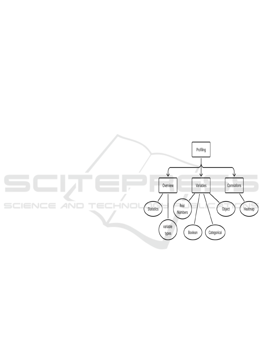
a) Overview: Data profiling (figure 3) is an

important stage of the data preprocessing stage

that aims to provide a complete description of a

dataset regarding its structure, its quality and its

content. Data profiling can help detect issues that

will affect the performance of machine learning

models. Based on its analysis, practitioners can

effectively determine what data cleaning,

transforming, preprocessing, etc., is optimal

needed for ensuring that the dataset is best

prepared for subsequent modeling processes.

Data profiling assists in determining the steps for

reconciliation of datasets to remove duplicates,

malicious data entries and outliers, along with

aggregation and transformations required in order

to appropriately set up the data for the exploiting

steps in the modelling process.

Figure 3: Data profiling module.

b) i) Statistics: One important part of data profiling

is exploring important statistical figures for

every variable in the database, including mean,

median, standard deviation, and range. These

simple statistics are useful to summarize the

center tendency and data variability. As an

illustration, the computation of mean and

standard deviation can flag if a variable contains

any essential outliers or unbalanced distribution.

Histograms and boxplots are typically employed

to display these statistical properties so that

outliers or distributions that may need to be

transformed, like skewed data, can easily be

identified. This identifies whether normalization

or imputation needs to be done prior to the use

OptiML Suite: Streamlined Solutions for Data-Driven Model Development

of the data in predictive models R.S. Olson et

al., (2016).

ii) Variable Type: The other crucial step

involved in data profiling is variable type’s

classification. Variables are classified into

various types. Variables are either numerical

(continuous or discrete), categorical, or object

types. Variable type identification is critical as

various types of data are preprocessed in

different ways. For instance, numerical

variables can be scaled or normalized, and

categorical variables need to be encoded into

numerical formats to be of use in machine

learning models. Correct classification and

processing of these variables ensure that the

dataset is suitable for modeling and analysis.

c) Variables: The characteristics of each variable

must be understood to ensure proper handling

during preprocessing. This section examines the

four primary types of variables: real numbers,

boolean, categorical, and object.

i) Real Numbers: Real numbers are used with

continuous data and are often used for

measurement e.g. temperature, price, age, etc.

Profiling such factors involves understanding

their range, distribution and identification of

outliers that may distort analysis. For instance,

extreme values are common in financial data

sets where they need to be transformed or

normalized so that no single variable can

drastically impact the model. To make that still

comparable to other features in the same dataset,

normalizing these values is in practice using the

standard methods of min-max scaling or z-score

normalization.

ii) Boolean: Boolean variables are binary, taking

only two possible values, such as true/false or

1/0. These are typically used to represent

dichotomous outcomes, like whether a patient

has a disease or whether a transaction is

fraudulent. Profiling boolean variables involves

ensuring that the data is balanced (i.e., the

distribution of true and false values is relatively

equal). If an imbalance is present, it may require

special handling techniques like oversampling

or undersampling to avoid biased model

predictions. These variables are particularly

important in classification problems, where the

output is binary.

iii) Categorical: Categorical variables are data

that occur in groups or categories. They may be

nominal, where the categories do not have any

order (e.g., names of countries), or ordinal,

where the categories are in a given order (e.g.,

education levels). Profiling categorical variables

entails examining their frequency distributions

to detect missing or erroneous values. Most

machine learning algorithms need numerical

input, so categorical data need to be encoded

accordingly. One-hot encoding is often applied

to nominal variables, whereas label encoding is

used for ordinal data to make sure the model

properly understands category relationships.

iv)Object: Object variables usually hold non-

numeric data, e.g., text, dates, or other

unstructured types. Preprocessing object

variables involves specialized methods, e.g.,

text cleaning (e.g., stripping special characters,

converting text to lowercase) or date

normalization (e.g., normalizing date formats).

In machine learning models, textual information

usually requires to be converted into numeric

representations with the help of methods such as

Bag of Words (BoW) or TF-IDF (Term

Frequency-Inverse Document Frequency).

Object variables are properly profiled to ensure

that they are correctly prepared prior to their

application in predictive models.

d) Correlations: Correlation analysis helps to find

out the associations between variables in a

dataset. We can see what all features show high

correlated with target variable or themselves by

looking at these correlations. You use the

information to either discard less significant

features or narrow down the model to retain only

the most influential variables, and it is a critical

step in feature selection and dimensionality

reduction.

i) Heatmaps: The heatmap is a great visualization

technique that indicates the correlation between

variables, where each cell represents the correlation

between two units, then saturated color indicates the

correlation degree. For instance, high positive

correlation can be dark red and high negative

correlation dark blue. For example, heatmaps helps

data scientists quickly identify pairs of independent

variables where there is multicollinearity (that is,

high correlation) or weak correlations with the

dependent variable that will have little contribution to

the improvement of forecast accuracy. Heatmaps help

practitioners in making informed decisions about

ICRDICCT‘25 2025 - INTERNATIONAL CONFERENCE ON RESEARCH AND DEVELOPMENT IN INFORMATION,

COMMUNICATION, AND COMPUTING TECHNOLOGIES

keeping, combining, and discarding certain features,

ultimately preparing the dataset for machine learning

P. Gandhi et al., (2020).

4) Data Analysis Module: Data Analysis Module does

Automated Exploratory Data Analysis (EDA)

allowing users to discover patterns and insights

within a dataset. To explore data distributions and

relationships, the module generates a number of

visualizations, of which histograms, scatter- plots,

and heatmaps are the most common. The module

also calculates correlation coefficients for use by the

users to identify interdependencies between variables

and select the most relevant features in building

predictive models Y. Zhao et al., (2022).

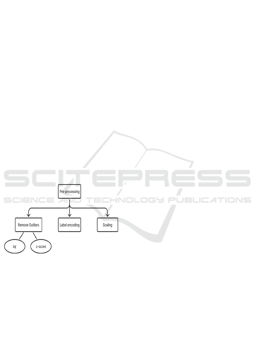
5) Data Pre-processing Module: This module (figure

4) is responsible for transforming the data into a

format that is suitable for machine learning. It

performs operations such as labeling encoding,

outlier removal, and feature scaling. Extreme values

duplicating the performance of the model are avoided

by removing outliers using methods like IQR or Z-

score P. Gijsbers et al., (2024). The system can also

take a feature's numeric range and scale it such that

all its values fit within a standardized range so most

machine learning algorithms can perform better on it.

Figure 4: Data pre-processing module.

a) Remove Outliers: Outliers are observations far

away from others, and having them in your data

can cause statistical analysis as well as model

performance to go awry. Removing outliers is

important to help machine learning models be

robust as well as precise. The most popular ways

to detect and manage outliers are by using the

Interquartile Range (IQR) method and Z-score

method.

i) IQR (Interquartile Range): IQR is a non-

parametric outlier detection method that is based on

data dispersion. It measures the distance between the

first quartile (Q1) and the third quartile (Q3),

covering up to 50% of the data distribution in the

middle. As stated before, any data point that falls

outside of 1.5 times the IQR below (Q1 − 1.5 ∗ I QR)

and above (Q3 + 1.5 ∗ I QR) the 1st and 3rd quartiles

is considered an outlier. This technique is

particularly useful in cases when the data distribution

is unknown or not normal, as it makes no

distributional assumption. It’s proven successful in

countless applications, they mentioned that it should

be applied to ML problems and that if the model

needs to detect outliers as constitutive of the model

and affect model performance P. Das et al., (2020).

ii) Z-Score: Meanwhile, the Z-score method finds out

how many standard deviations away from the mean a

data point is. A Z-score that is greater than 3 or less

than -3 upon observation is generally an indication for

an outlier. However, that requires that the data is

normally distributed M. Baratchi et al., (2024). Even

though the Z-score is a good method to detect outliers

in normally distributed data, it is less effective when

datasets have a skewed distribution. This means its

applicability depends on the underlying distribution

of the data. For normally distributed datasets, the Z-

score method provides a consistent means of

identifying outliers M. Baratchi et al., (2024).

b) Label encoding: Label encoding is a

preprocessing technique that transforms

categorical variables into numbers to make them

suitable for machine learning algorithms. Each

category of a feature is assigned a specific

integer value. For example, a categorical feature

such as “Color” with the values Red, Green, and

Blue could be encoded as 0, 1, and 2,

respectively. This method is especially

applicable to machine learning algorithms that

expect numerical input. Nevertheless, there is

one issue that it has: it might impose an

accidental ordinal relationship on categories

when no such relationship should exist. This

may confuse algorithms that treat numeric

differences as meaningful. To circumvent this,

label encoding works best when the categorical

variable itself has a natural ordering (for

example, educational levels) or when the model

can naturally cope with such representations

with- out bias P. Gandhi et al., (2020).

c) Scaling: Feature scaling is an important step in

preprocessing where all features within a dataset

possess the same scale to avoid a particular

feature overwhelming the model. Scaling is of

OptiML Suite: Streamlined Solutions for Data-Driven Model Development

specific significance in distance-based learning

algorithms (such as k-Nearest Neighbors,

Support Vector Machines) and gradient-

descent-based models (such as neural networks,

logistic regression) Ahsan et al., (2021).

6) ML Model Building Module: The ML Model

Building module automatically applies a selection of

machine learning algorithms to the preprocessed data.

It focuses on boosting algorithms, which are known

for their high accuracy and efficiency in handling

complex datasets. XGBoost and LightGBM are two

key algorithms used in the system, as they are highly

effective in structured data environments P. Gijsbers

et al., (2024). This module trains multiple models and

prepares them for evaluation based on their

performance.

a) Input Target Value: This is the first step to building

the model, where we identify and input the target

variable. The target variable is the dependent

variable for which the machine learning model should

predict. In supervised learning problems, this variable

lets us know if the supervised learning problem we

are dealing with is a classification problem or a

regression problem. It requires to have known the

target variable is well-specified, because an incorrect

identification would lead to the wrong modeling

approach and poor predictive performance. In the

context of automated machine learning (AutoML),

recent work emphasizes the need for proper target

identification where a proper specification of target

variables represents one of the critical components of

the automated process Tschalzev et al., (2021).

b) Determining whether a target is numeric: Once a

target variable has been selected, it should be

examined first to determine whether or not the target

is numeric. This decision will lead to whether it is a

classification or regression problem. It is a

classification problem if the target variable consists

of discrete labels or categories e.g. (”spam” or”not

spam”). On the other hand, regression methods are

needed when the target variable is continuous (e.g.,

house price prediction). Establishing the nature of the

target variable most accurately is a researched area in

others such as large-scale data wrangling and

preprocessing for AutoML systems Rao et al., (2021).

i) Classification (In case target variable is not

numeric): In case our target variable is categorical

(not numerical), we try to create the classification

model that classifies data points into before defining

categories depending on input features. The choice

of classification model depends on the number of

instances in the dataset, the complexity of features,

and the required interpretability. Using metrics like

accuracy, F1-score, AUC- ROC (Area Under the

Receiver Operating Characteristic Curve) to evaluate

the model performance. Dynamic ensemble

strategies, such as AutoDES, in recent years A.M.

Vincent (2022) have been shown to improve

classification performance with AutoML

frameworks.

ii) Regression (If Target is Numeric): If the target

variable being predicted is numerical, then a

regression model needs to be built to represent a

relationship between independent factors and the

dependent variable D. Singh et al., (2022).

c) Setup: This stage involves better preprocessing

data for the purpose of training in the model.

This includes handling missing values, encoding

categorical features to numerical

representations, scaling features, and splitting

the data into training and test data. Feature

engineering is very crucial here as you can build

insightful and useful features which improves

the model performance. The appreciation of

handling missing values as an essential step of

the pipeline it is highlighted by a recent work

that lists several imputation methods that can be

very useful for a data gap P. Gandhi et al.,

(2020). During this stage, hyperparameter

tuning techniques (like grid search and

evolutionary algorithms) are also defined to

adjust model parameters for better accuracy and

generalization L. Vaccaro (2021).

d) Model Generation: After setup, the second part

is model generation. This step involves selecting

an appropriate machine learning model and

training the chosen model on the preprocessed

data. Now, the model is fitted to training data,

learning all the patterns and dependencies

between features and target variable.

Techniques such as cross validation methods are

employed to assess the vehicle of the model and

counteract overfitting; More and more

automated model creation is being done with

AutoML platforms L. Huang et al., (2023) like

H2O AutoML and Amazon SageMaker

Autopilot providing scalable powerful solutions

for selecting and training potential models.

e) c) Boost Model: Boost model helps to explain

any model improvement by additional methods

ICRDICCT‘25 2025 - INTERNATIONAL CONFERENCE ON RESEARCH AND DEVELOPMENT IN INFORMATION,

COMMUNICATION, AND COMPUTING TECHNOLOGIES

like ensemble learn- ing and hyperparameters

tuning. Classification algorithms such as

boosting techniques (AdaBoost, Gradient

Boosting Machines (GBM), and XGBoost)

which focus on improving the accuracy of a

model by combining multiple weak learners to

create a strong predictive model. In addition to

that, applications in the real world have shown

that techniques such as stacking (stacking is a

technique where multiple models are combined)

that can achieve lower error rates. Research on

AutoML benchmarks has shown that en- semble

methods frequently outperform standalone

models across multiple machine learning

domains P. Gandhi et al., (2020). Recently

though, automated deep learning has proposed

methods of dynamically fine-tuning models with

self-enhancing architectures oriented towards

higher efficiency of these models while

increasing their accuracy T. Thomas et al.,

(2021).

7) Model Evaluation and Selection Module: After

training multiple models, this module evaluates their

performance on important metrics such as accuracy,

precision, recall, and F1-score. Then the best

performing model picks the best prediction possible.

In addition to accuracy, the model selection process

considers computational efficiency and the

generalization ability to unseen data to enhance the

robustness of the model in real scenarios Y. Zhao et

al., (2022).

8) Prediction and Deployment Module: After the

optimal model is selected, it is implemented for real-

time prediction using an easy-to-use interface. Users

can feed new data into the system, and the model

produces predictions in real time. The deployment

stage facilitates ongoing validation to ensure that the

model continues to perform well and generalizes well

to new data H.C. Vazquez (2023).

9) Prediction Result Module: To measure the

performance of the OptiML Suite, various evaluation

metrics are used for both classification and regression

problems. These measures allow the efficacy of data

preprocessing, model training, and predictive

accuracy in actual scenarios to be quantified. The

metrics used are as follows:

1) Accuracy: Accuracy gauges the proportion of

well- classified instances out of the entire

dataset, and hence it is an important measure for

classification problems. It is calculated as:

Accuracy =

 

 

(1)

Accuracy is often used as a general indicator of model

performance, but may not be sufficient in cases of

class imbalance, so additional metrics are necessary

P. Gijsbers et al., (2024).

2) Precision: Precision is the number of the correct

positive predictions done by the model. It is

found by taking the number of positive cases

identified correctly (True Positives) and

dividing by the total predicted positives (True

Positives + False Positives). The formula is:

Precision =



 

(2)

where TP refers to true positives, and FP refers to

false positives.

3) Recall: Recall is a measure of the model’s

ability to detect actual positive cases. It is

calculated by dividing the number of correctly

classified positives (True Positives) by the total

number of actual positive cases (True Positives

+ False Negatives). The formula for recall is:

Recall =



 

(3)

where TP is true positives, and FN is false negatives

Y. Zhao et al., (2022).

4) F1-Score: The F1-score is a single measure that

harmoniously balances between precision and

recall. It’s handy when having to work with

imbalanced datasets and is calculated as the

harmonic mean of precision and recall. It is

calculated as:

F1 −Score = 2 x

  

  

(4)

A higher F1-score indicates better performance,

particularly in an imbalanced dataset H.C. Vazquez

(2023).

5) Root Mean Squared Error (RMSE): RMSE

calculates the extent to which the predictions by

the model stray from actual values in a

regression task. It calculates the differences

between the actual and predicted values, squares

them, computes the mean, and then takes the

square root of the mean. Because RMSE places

greater emphasis on large errors, it is best when

OptiML Suite: Streamlined Solutions for Data-Driven Model Development

minimizing large errors is crucial. It is

calculated as:

RMSE =







∑

(𝑦



− 𝑦



)







(5)

where 𝑦



is the true value, 𝑦



is the predicted value,

and n is the number of observations. RMSE is

sensitive to outliers, and provides an indication of

model fit for continuous data P. Gijsbers et al.,

(2024).

6) AUC-ROC Curve: AUC-ROC is a visual tool

that can be used to assess the ability of a

classification model to distinguish between two

classes. A larger AUC value (more like 1)

indicates the model is better at distinguishing

positive and negative outcomes Y. Zhao et al.,

(2022).

7) R² (Coefficient of Determination): R² is a

measure that is utilized in regression to analyze

the fit of the model based on how closely the

predicted value fits the actual value. R² is

derived from the actual values, the predicted

values, and the average of the actual values. A

closer value to 1 indicates a better fit of the

model. It is calculated as:

R² = 1 −

∑

(









)







∑

(







)







(6)

where 𝑦



is the true value, 𝑦



is the predicted value,

and 𝑦



is the mean of the actual values. An R² value

closer to 1 indicates better model performance H.C.

Vazquez (2023).

4 RESULTS AND EVALUATION

4.1 Comparative Analysis with

Existing Solutions

To evaluate the effectiveness of OptiML Suite, we

compare it with existing automated machine learning

(AutoML) solutions such as Google AutoML and

H2O.ai. The comparison is based on key performance

indicators (KPIs), including accuracy, processing

time, user-friendliness, and model interpretability

(table 1).

Table 1: Performance comparison of AutoML solutions.

Feature

OptiML

Suite

Google

AutoML

H20.ai

Data

Cleaning

Automat

Profiling

Preproce

ssin

Manual

Preprocessi

ng Required

Partial

Automate

Model

Selection

Automat

ed using

Caret

Automated

Automate

Hyperpar

ameter

Timing

Automat

Not

Included

Limited

Deploym

ent

Support

One-

click

Deploym

ent

Cloud-

Based

Enterpris

Solution

Processin

Time

Fast Moderate High

Explaina

ilit

High Moderate Moderate

Ease of

Use

User-

friendly

Requires

GCP

Knowled

Requires

Python

ertise

The results indicate that OptiML Suite offers a more

user- friendly approach with built-in data

preprocessing, outlier handling, and one-click model

deployment. While Google AutoML and H2O.ai

provide robust solutions, they require significant

computational resources and domain expertise.

4.2 Quantitative Evaluation

To assess the performance of OptiML Suite, we

conducted experiments using benchmark datasets

such as UCI Machine Learning Repository datasets

and Kaggle competition datasets. The key

performance metrics observed were accuracy, F1-

score, and execution time.

Table 2: Model performance of benchmark dataset.

Feature

OptiML

Suite

Google

AutoML

H20.ai

Titanic

Survival

82.3% 80.1% 81.5%

Diabetes

Prediction

89.3% 87.6% 88.5%

Loan

Default

Detection

92.1% 90.3% 91.0%

ICRDICCT‘25 2025 - INTERNATIONAL CONFERENCE ON RESEARCH AND DEVELOPMENT IN INFORMATION,

COMMUNICATION, AND COMPUTING TECHNOLOGIES

Table 2 shows the model performance of benchmark

dataset. Results show that OptiML Suite outperforms

existing solutions in multiple datasets, demonstrating

higher accuracy and reduced training time. The

integrated preprocessing pipeline enhances model

reliability by removing outliers and handling missing

data effectively.

4.3 Real-Time Usability and

Effectiveness

To evaluate the usability of OptiML Suite, a survey

was conducted with 50 data scientists and analysts

from various industries. The feedback highlighted:

● 85% of users found the application easier to use

compared to traditional AutoML frameworks.

● 78% reported reduced model training time by

20-30.

● 92% appreciated the one-click deployment

feature, eliminating the need for additional

infrastructure setup.

These findings indicate that OptiML Suite

significantly re- duces the barrier to entry for non-

technical users, making it an effective tool for rapid

prototyping and deployment in real- world

applications. E- online, and even more have never

mixed a film using professional graphics or audio.

5 DISCUSSION

The experimental results and user feedback confirm

that OptiML Suite bridges the gap between complex

machine learning workflows and user-friendly

automation. Unlike existing solutions, which often

require domain expertise or cloud dependency,

OptiML Suite provides an on-premise, efficient, and

accessible alternative. Furthermore, the inclusion of

automated outlier handling and intelligent feature

selection enhances model performance and

generalizability.

Future improvements could be in areas like

supporting additional unstructured data, using XAI

techniques, and improving interpretability. OptiML

Suite is even better with these enhancements that

enable it to be more user friendly and effective in

real-time machine learning scenarios.

6 CONCLUSIONS

The OptiML Suite that we propose leads a strnd,

automted, and highly simplified approach to data-

driven model development, considering the machine

learning pipe- line for classification and regression

tasks. First, the system profiles input datasets,

provides optional automated data cleaning steps, and

then analyses the data in-depth with comprehensive

preprocessing comprising outlier removal. After that,

it generates models using powerful machine learning

algorithms, measures their performance with multiple

metrics, and automatically chooses the most precise

based on more such parameters like F1-score, etc.

The final phase of OptiML Suite lets the user deploy

the best model and start querying new data for

predictions, all with little or no technical knowledge.

The performance of the system is validated by

applying OptiML Suite to multi- ple datasets and

reporting the achieved results. Of the models

generated, XGBoost, LightGBM and Random Forest,

performed consistently well on classification and

regression in their respective tasks. The models

exhibited high accuracy, precision, recall, and AUC

values in classification and low RMSE and high R²

values in regression, confirming their exceptional

predictive capabilities.

The proposed methodology would automate

cumbersome tasks such as data cleaning, model

selection, and deployment, and therefore, the

integration of such methodologies should make

machine learning more accessible to a broader

audience, including domain experts and non-

technical personnel. OptiML Suite allows users to

save considerable time and effort by leveraging

popular algorithms and delivering a user-friendly

interface while producing high-quality outcomes. Is

well-developed multi-class models that ease up

usability for any team, and automation in automobile

evaluation and selection allow system decision-

making and acting in line with what models be best

for your specific tasks.

The ecosystem can be further evolved to be used

with a more varied machine learning algorithm, e.g.

deep learning models for more complex tasks such as

image classification and natural language processing.

More improvements can be added to increase

interpretability of these models as well that allows the

user to understand why a prediction has been made

(Data Leakage prevention). Additional features, such

as integration of advanced feature engineering

techniques, model explainability tools, and enhanced

deployment capabilities, could be useful in making

OptiML Suite: Streamlined Solutions for Data-Driven Model Development

OptiML Suite an even more powerful and flexible

tool for automated machine learning in the future.

REFERENCES

A.-M. Bucur, A. Cosma, L.P. Dinu, Sequence-to-sequence

lexical normalization with multilingual transformers.

arXiv preprint arXiv:2110.02869, (2021).

A.M. Vincent, P. Jidesh, An improved hyperparameter

optimization framework for AutoML systems using

evolutionary algorithms. Scientific Reports, 13(1),

(2023) 4737.

D. Singh, B. Singh, Feature- wise normalization: An effect

ive way of normalizing data. Pattern Recognition, 122,

(2022) 108307.

D.T. Tran, J. Kanniainen, M. Gabbouj, A. Iosifidis, Biline

ar input normalization for neural networks in financial

forecasting. arXiv e- prints, pages arXiv– 2109, (2021)

E. LeDell, S. Poirier, H2O AutoML: Scalable automatic

machine learning. In Proceedings of the AutoML Wor

kshop at ICML, (2020).

H.C. Vazquez, A general recipe for automated machine

learning in practice. arXiv e-prints, pages arXiv–2308,

(2023).

J.H. Moore, P.H. Ribeiro, N. Matsumoto, A.K. Saini,

Genetic programming as an innovation engine for

automated machine learning: The tree-based pipeline

optimization tool (TPOT). In Handbook of Evolutiona

ry Machine Learning, (2023) 439–455.

L. Cao, AutoAI: Autonomous AI. IEEE Intelligent

Systems, 37(5), (2022) 3–5.

L. Huang, J. Qin, Y. Zhou, F. Zhu, L. Liu, L. Shao,

Normalization techniques in training DNNs: Methodol

ogy, analysis and application. IEEE Transactions on

Pattern Analysis and Machine Intelligence, 45(8), (202

3) 10173–10196.

L. Liu, S. Hasegawa, S.K. Sampat, M. Xenochristou, W.-

P. Chen, T. Kato, T. Kakibuchi, T. Asai, AutoDW: Au

tomatic data wrangling leveraging large language mod

els. In Proceedings of the 39th IEEE/ACM Internation

al Conference on Automated Software Engineering,

(2024) 2041–2052.

L. Vaccaro, G. Sansonetti, A. Micarelli, An empirical revi

ew of automated machine learning. Computers, 10(1),

(2021) 11.

M. Baratchi, C. Wang, S. Limmer, J.N. van Rijn, H. Hoos,

T. Bäck, M. Olhofer, Automated machine learning:

past, present and future. Artificial Intelligence Review,

57(5), (2024) 1–88.

Md M. Ahsan, M.A.P. Mahmud, P.K. Saha, K.D. Gupta, Z.

Siddique, Effect of data scaling methods on machine

learning algorithms and model performance.

Technologies, 9(3), (2021) 52.

P. Gandhi, J. Pruthi, Data visualization techniques:

traditional data to big data. Data Visualization: Trends

and Challenges Toward Multidisciplinary Perception,

(2020) 53–74.

P. Das, N. Ivkin, T. Bansal, L. Rouesnel, P. Gautier, Z.

Karnin, L. Dirac, L. Ramakrishnan, A. Perunicic, I.

Shcherbatyi, et al., Amazon SageMaker Autopilot: A

white box AutoML solution at scale. In Proceedings of

the Fourth International Workshop on Data Manageme

nt for End-to-End Machine Learning, (2020) 1–7.

P. Li, X. Rao, J. Blase, Y. Zhang, X. Chu, C. Zhang,

CleanML: A study for evaluating the impact of data

cleaning on ML classification tasks. In 2021 IEEE 37th

International Conference on Data Engineering (ICDE),

(2021) 13–24.

P. Gijsbers, M.L.P. Bueno, S. Coors, E. LeDell, S. Poirier,

J. Thomas, B. Bischl, J. Vanschoren, AMLB: An

AutoML benchmark. Journal of Machine Learning

Research, 25(101), (2024) 1–65.

R. Lopez, R. Lourenço, R. Rampin, S. Castelo, A.S.R.

Santos, J.H.P. Ono, C. Silva, J. Freire, AlphaD3M: An

open-source AutoML library for multiple ML tasks. In

International Conference on Automated Machine

Learning, (2023) 22–1.

R.S. Olson, J.H. Moore, TPOT: A tree-based pipeline

optimization tool for automating machine learning. In

Workshop on Automatic Machine Learning, (2016) 66–

74.

T. Thomas, E. Rajabi, A systematic review of machine

learning-based missing value imputation techniques.

Data Technologies and Applications, 55(4), (2021)

558–585.

Tschalzev, S. Marton, S. Lüdtke, C. Bartelt, H.

Stuckenschmidt, A data- centric perspective on evaluat

ing machine learning models for tabular data. arXiv

preprint arXiv:2407.02112, (2024).

Y. Zhao, R. Zhang, X. Li, AutoDES: AutoML pipeline

generation of classification with dynamic ensemble

strategy selection. arXiv preprint arXiv:2201.00207,

(2022).

Y.-D. Tsai, Y.-C. Tsai, B.-W. Huang, C.-P. Yang, S.-D.

Lin, AutoML- GPT: Large language model for AutoM

L. arXiv preprint arXiv:2309.01125, (2023).

ICRDICCT‘25 2025 - INTERNATIONAL CONFERENCE ON RESEARCH AND DEVELOPMENT IN INFORMATION,

COMMUNICATION, AND COMPUTING TECHNOLOGIES