Detection and Prediction of Primary Productivity in Coastal

Environment Using Ensemble Models

R. Sivaranjini

and Sharanya S

Department of Computer Science & Engineering, SRM Institute of Science & Technology, Kattankulathur, Chennai, Tamil

Nadu, India

Department of Data Science and Business Administration, SRM Institute of Science & Technology, Kattankulathur,

Chennai, Tamil Nadu, India

Keywords: Algae Bloom, CNN, HCNN, LSTM, Convolutional LSTM, Autoencoders.

Abstract: Prediction on marine productivity in the ecosystem is a challenging task nowadays. Fault prediction in

marine ecosystem occurs due to the climate change, waste water infusion in the marine environment which

leads to the harmful primary production in the marine ecosystem. In traditional method it was a struggle to

focus on the complexity and the changes in the variation metrices. To overcome those complexity deep

learning acts as a powerful tool to predict modelling methods in various domains. Deep learning algorithm

mainly has an ability to differentiate patterns from huge dataset. This study empirically analyses the

effectiveness of various deep learning algorithm used to analyse prediction in primary productivity mainly

focusing on algae bloom. General key performance metrices like accuracy, recall, precision and F1 score are

analysed. The algorithms like Convolutional Neural Network (CNN) and Hybrid Convolutional Neural

Network (HCNN) are the superior models in predicting accuracy when compared to traditional methods.

Overall, this study focuses on the use of various deep learning algorithm which can be implemented to

analyse the algae bloom in marine ecosystem. This concept will be helpful for the readers focusing on Algae

Bloom.

1 INTRODUCTION

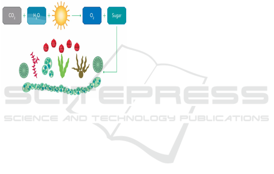
Primary productivity is the rate at which

photosynthetic organisms such as plants and algae

convert energy into organic molecules through the

photosynthesis process. Using sunlight, this process

transforms carbon dioxide and water into glucose

and creates oxygen. The generated organic

substances supply nutrition to rest of the ecosystems.

1.1 Environmental Value of Main

Productivity

In marine ecosystems, primary production

constitutes the base of the food chain. Where the

Producers or autotrophic organisms changes the

solar energy into chemical form which is later

passed on to herbivores and predators within the

ecosystem.

During Photosynthesis Primary producers

combines nutrients like carbon, nitrogen, and

phosphorus into their tissues. These nutrients are

returned into the environment when these nutrients

are consumed and broken down by other species or

by natural processes, hence encouraging nutrient

cycling in ecosystems.

Production of Oxygen: The major function of

photosynthesis is oxygen creation. Most living

organisms depends on atmospheric oxygen levels,

which plants and algae considerably contribute in

releasing oxygen as a byproduct while they make

glucose for their energy level.

Carbon dioxide from the atmosphere is taken by

the Primary producers during photosynthesis, hence

changes occurs in the global carbon cycle. This

absorption influences atmospheric carbon dioxide

levels, consequently impacting the Earth's

temperature and global climate patterns.

Main production is also incredibly vital for

human civilizations since it produces food, fiber,

fuel, and pharmaceuticals among other requirements.

Direct or indirectly dependant on productive

ecosystems include fishing, agriculture, forestry, and

ecotourism.

Sivaranjini, R. and S., S.

Detection and Prediction of Primary Productivity in Coastal Environment Using Ensemble Models.

DOI: 10.5220/0013909000004919

Paper published under CC license (CC BY-NC-ND 4.0)

In Proceedings of the 1st International Conference on Research and Development in Information, Communication, and Computing Technologies (ICRDICCT‘25 2025) - Volume 4, pages

115-124

ISBN: 978-989-758-777-1

115

1.2 Field dimensions

Direct monitoring of oxygen production by primary

producers (e.g., aquatic plants, phytoplankton)

employing techniques including light and dark bottle

tests. This requires monitoring fluctuations in

dissolved oxygen concentrations in under control

situations.

Direct monitoring of biomass building and

growth rates of key producers are done across time.

This generally requires measuring biomass using

growth chambers or harvesting and weighing plant

materials. The figure 1 shows Algal Bloom process.

Figure 1: Algal Bloom process.

2 RELATED SURVEYS

This survey focusses on the application and

methodologies that were implemented by various

researchers in marine environment.

Deep learning for marine species recognition was

proposed by Lian Xu et al focus on deep learning

techniques that are used to identify automatically the

species in marine environment. The author

implements CNN to overcome the challenges that

are faced by the traditional methods. With the help

of CNN, the author analysed underwear imagery and

acoustic data. With this analysis he classified the

data according to their characteristics.

Deep learning and transfer learning features for

plankton classification, Alessandra Lumni et al uses

deep learning techniques to differentiate plankton.

Author uses transfer learning, pre-tuning and fine-

tuning models o train the model. Ensemble model is

proposed by the author to improve the performance.

CNN method is implemented for identification of

plankton.

Defining a procedure for integrating multiple

oceanographic variables in ensemble models of

marine species distribution, D. Panzeri et al focus

five different modelling approaches. For each

approach different spatial data and test data set is

used to enhance performance. Depth, spatiotemporal

variables are used as input for simple model and

Oceanographic variables are used for complex

model. The author focusses on space and time on

European lake.

Species distribution modelling for machine

learning practitioners, Sara Beery et al here in his

work the author implemented SDM Species

Distribution Modelling to focus where the huge

number species were found in the marine ecosystem.

This modelling used to predict the spatial and

temporal patterns of species.

There are lot of work are done in the filed of

marine environment focusing on Algal Bloom and

however there are lot of limitations too.

2.1 Preprocessing and Data Gathering

2.1.1 Data Gathering

There are several sources from which primary

productivity data can be measured and monitored.

Some of the common sources are listed for obtaining

primary productivity data.

2.1.2 Satellite Imagery

Measuring vegetation indicators like Normalized

Difference Vegetation Index (NDVI) and Enhanced

Vegetation Index (EVI) are done with the help of

Moderate Resolution Imaging Spectroradiometer

(MODIS) which provides global coverage.

NDVI = (NIR — VIS)/ (NIR + VIS)

[13]

EVI = G * ((NIR - R) / (NIR + C1 * R – C2 * B

+ L))

[14]

Another method is Landsat which gives higher

spatial resolution than MODIS, suitable for complete

land cover and vegetation dynamic monitoring.

2.1.3 Satellites in Ocean Colour

Measuring ocean colour to estimate concentration of

chlorophyll-a is monitored using Sea-Viewing Wide

Field-of- View Sensor (SeaWiFS). Hence

phytoplankton biomass and marine algal bloom can

be measured. The figure 2 shows Satellite image by

SeaWiFs for Algal detection

ICRDICCT‘25 2025 - INTERNATIONAL CONFERENCE ON RESEARCH AND DEVELOPMENT IN INFORMATION,

COMMUNICATION, AND COMPUTING TECHNOLOGIES

116

Figure 2: Satellite image by SeaWiFs for Algal detection.

2.1.4 Field Measurements

Chamber-based methods allow to analyse

photosynthesis rates of plants or algae. Often

employing gas exchange measurements to estimate

carbon dioxide absorption and oxygen production,

Gathering plant or algal samples to measure biomass

growth over time is the biomass harvesting method.

Tracks carbon absorption and integration into

organic matter using isotopically labelled carbon

dioxide (e.g., ^14C).

2.1.5 Environmental and Climate Data

Recording information on temperature, precipitation,

solar radiation, and other environmental conditions

impacting major production are analysed with the

help of meteorological stations.

Soil Measurements is used to identify the soil

characteristics including nutrient content, pH, and

moisture levels that impact plant growth and

production effects. The figure 3 shows

Environmental and climate change image.

Figure 3: Environmental and climate change image.

2.2 Remote Sensing Products and

Database

To access a wide range of satellite data products,

including MODIS, Landsat, and other remote

sensing datasets NASA Earth Observing System

Data and Information System (EOSDIS) provides

large dataset in real time.

European Space Agency (ESA) Earth

Observation Data offer satellite data for monitoring

land and ocean conditions essential to primary

production.

2.2.1 Data Preprocessing

Getting major productivity data available for deep

learning models relies crucially on data preparation.

Typical cleaning, preprocessing, and data

preparation techniques are discussed.

2.2.2 Data Cleansing

Managing Missing Values: Find and fix missing data

points. Strategies like imputation using mean,

median, or mode or deletion of incomplete records

may be utilized dependent on the dataset and nature

of missing information.

Look for outliers that might alter the data

distribution or impair model performance. Statistical

tools (e.g., z-score) or domain-specific knowledge

may assist one to locate outliers.

To boost model training convergence,

normalization /standardization is used to size

numerical features to a similar range. Common

strategies include standardizing (scaling to zero

mean and unit variance) or min-max scaling (scaling

to [0, 1].

2.2.3 Data Translation

Feature engineering extract new features from

present ones maybe enhancing model performance.

Regarding major productivity, this can involve

aggregating meteorological variables (e.g., monthly

averages) or calculating vegetation indices from

satellite data (e.g., NDVI, EVI).

To minimize noise and capture long-term trends,

temporal aggregation is used to aggregate daily

measurements which converts into meaningful

intervals either monthly or seasonal averages.

Using interpolation methods e.g., bilinear

interpolation aligns spatial resolutions of various

datasets (e.g., satellite pictures, climate data) to a

same grid or resolution.

Detection and Prediction of Primary Productivity in Coastal Environment Using Ensemble Models

117

2.2.4 Information Integration

Integrate various datasets e.g., satellite photos,

temperature data, ground measurements into a

cohesive dataset appropriate for deep learning

models. Throughout merging, maintain uniformity in

timestamps, geographical locations, and data

formats.

While lowering dimensionality and

computational complexity, pick important qualities

that most assist to forecast major production. Feature

selection may benefit from approaches including

feature significance from machine learning models

or correlation analysis from statistical models.

2.2.5 Split Data

Creates various set of data for training, validation,

and testing from the given dataset. The deep learning

model is trained using the training set; the validation

set sets hyperparameters and records model

performance; the test set analyses the final model

performance on unprocessed data.

For time-dependent data that instance, seasonal

swings in primary productivity ensure that training

and testing datasets are split in a method that

respects temporal dependencies and mimics real-

world deployment conditions.

2.2.6 Getting Model Training Input Data

Transpose data into representations suited for deep

learning models (like tensors for neural networks).

Make that input features suit the specified deep

learning framework (e.g., TensorFlow, PyTorch) and

are correctly ordered.

Considering hardware restrictions (e.g., GPU

RAM), partition the training data into batches to

facilitate efficient model training and optimization.

Following these preprocessing strategies enables

to ensure correct cleaning, transformation, and

integration of essential productivity data for training

deep learning models. Appropriately produced data

boosts the generalizability, accuracy, and reliability

of models used to predict primary output in

ecosystems.

3 FEATURE REVIEW

When anticipating primary production, feature

engineering is particularly crucial in increasing the

performance of deep learning models. Several other

variables or qualities acquired from the data can

potentially boost model performance.

3.1 Vegetational Indices

Calculated using satellite photographs to assess

green vegetation, Normalized Difference Vegetation

Index are sensitive to differences in canopy structure

and chlorophyll content, NDVI is a robust indication

of photosynthetic activity and primary production.

Designed to limit atmospheric influences and soil

background changes, Enhanced Vegetation Index

(EVI) like NDVI but delivers a more accurate

assessment of vegetation density.

3.2 Variables of Climate and Weather

Over various periods e.g., the growth season

average, maximum, or lowest temperatures impact

photosynthetic rates and plant development.

Rainfall frequency and quantity affects soil

moisture levels and nutrient availability,

consequently influencing plant yield.

Incoming light energy effects photosynthetic rate

as well as overall plant growth.

3.3 Land Surface Features

Using satellite data or land use maps enables one to

identify land cover types (e.g., woodlands,

grasslands, croplands) in respect to key productivity

variations.

Terrain characteristics like height, slope, and

aspect effect microclimatic conditions and water

availability, consequently impacting plant growth.

3.4 Attributes of Soil

Soil Moisture- The quantity of moisture in the soil

impacts plant water stress and nutrient absorption,

consequently impacting major production.

Plant growth and biomass building are regulated

by differences in nitrogen, phosphorus, potassium,

and other important nutrients.

3.5 Phenological Measurements

The length of the growth season is, the duration of

favourable conditions for plant development affects

output patterns.

Satellite data enables one to calculate time of leaf

emergence and senescence, hence revealing seasonal

variations in vegetation activity.

ICRDICCT‘25 2025 - INTERNATIONAL CONFERENCE ON RESEARCH AND DEVELOPMENT IN INFORMATION,

COMMUNICATION, AND COMPUTING TECHNOLOGIES

118

3.6 Metrics Derived from Satellite Data

Patterns and variability in vegetation indicators

across time for example, seasonal patterns,

anomalies to capture changes in primary output.

Spatial heterogeneity in vegetation indices or

climatic factors allows comprehension of landscape-

scale processes and ecosystem productivity

gradients.

4 DEEP LEARNING

ALGORITHMS

Several aspects including data type (e.g., satellite

imagery, time series data), computational resources,

and unique research purposes impact the choice of

deep learning architectures for assessing key

productivity. These are several common deep

learning architectures that might fit.

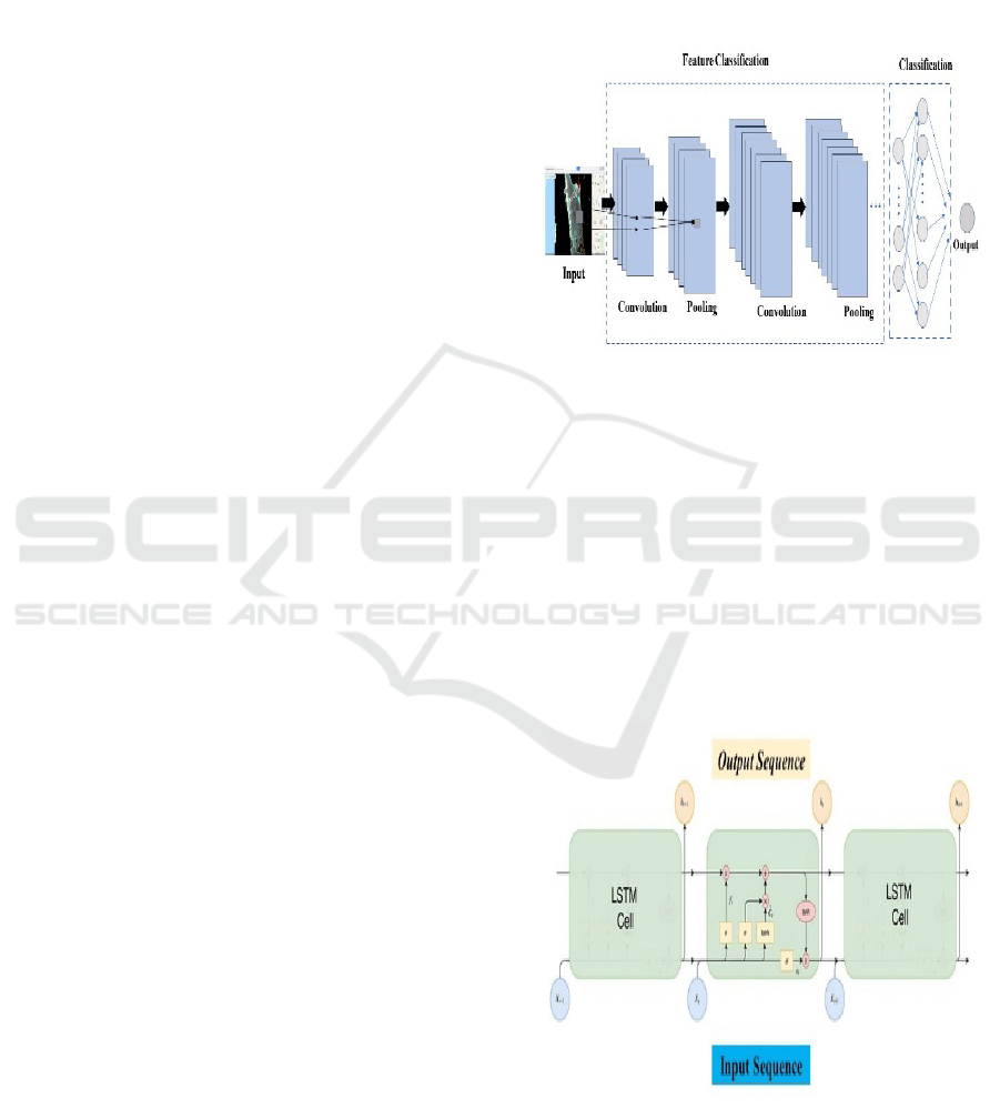
4.1 Convolutional Neural Networks

(CNN)

CNNs are ideal for analysing spatial data like land

cover maps or satellite photos. Usually containing

convolutional layers for feature extraction, pooling

layers for spatial down sampling, and fully

connected layers for classification or regression,

architecture. Effective capture of spatial

dependencies and patterns makes one robust to

spatial transformations and fluctuations.

Accepts input data usually satellite pictures or

other spatial data shown as multi-channel tensors

(e.g., RGB channels for imaging). Convolutional

layers enable you capture spatial patterns by means

of feature extraction utilizing convolutional filters.

Every layer employs a set of filters then activates

using functions. ReLU (Rectified Linear Unit) is

commonly employed because of its efficiency and

aptitude to handle sparse gradients. Down sample

feature maps to smaller spatial dimensions while still

keeping considerable information using pooling

layers. For usage in fully connected layers, flattening

layer turns 2D feature maps into a 1D vector.

Fully Connected (Dense) Layers: Handle the

flattened features for either classification or

regression operations. Usually employing a softmax

activation for classification or a linear activation for

regression, Layer creates predictions.

Randomly marks a fraction of input units to zero

during training to avoid overfitting and increase

generalization. The figure 4 shows convolutional

Neural Network.

Normalizing input data throughout the mini-

batch, batch normalisation stabilises and speeds up

the training process. Penalizes large weights to

prevent overfitting and model complexity.

Figure 4: Convolutional Neural Network.

4.2 Long Short-Term Memory (LSTM)

Appropriate for time series data includes primary

production temporal patterns, phenological metrics,

or climatic influences. RNNs and LSTMs handle

sequential input by way of recurrent connections,

hence capturing temporal relationships and patterns

across time. Suitable for prediction and anomaly

detection in time series data, advantages include

managing variable-length sequences and keeping

remembrance of earlier inputs.

Figure 5: LSTM.

Accepts sequential data containing temporal

trends in key productivity or climatic variable time

Detection and Prediction of Primary Productivity in Coastal Environment Using Ensemble Models

119

series. Process sequential input data in LSTM (or

RNN) Layers retaining a memory state to capture

temporal dependencies. Often utilized tanh or

sigmoid activations inside LSTM cells to modulate

information flow. Based on the studied sequence

data it generates predictions.

Applied to LSTM (figure 5) cell input and

recurrent connections, Dropout helps to decrease

overfitting and boost model generalization. L2

Regularization: Possibly employed to penalize

network's large weights.

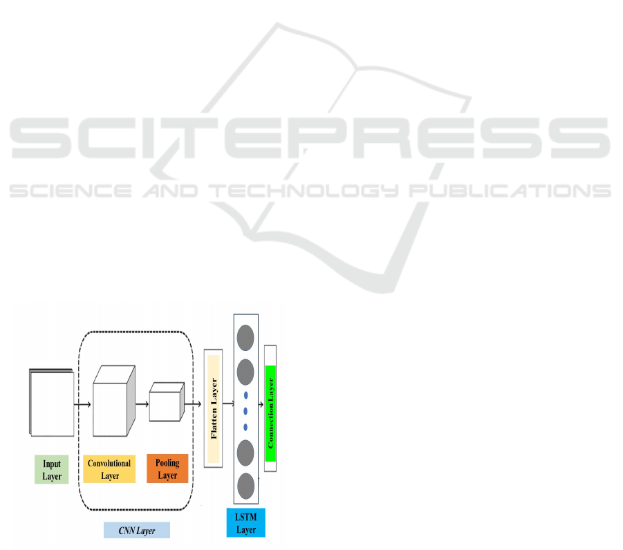
4.3 Convolutional-LSTM

Ideal for spatiotemporal data analysis, application

blends spatial and temporal linkages. Combining

CNNs with LSTM cells lets the model learn spatial

patterns via convolutional operations and temporal

dynamics via recurrent connections. Effective for

evaluating key production trends considering both

geographical and temporal interactions, it also aids

satellite-derived data with both spatial and temporal

dimensions.

Like in a normal CNN, convolutional layers

extract spatial information from incoming data.

Replace standard pooling layers with LSTM cells to

incorporate temporal dependencies and enable the

model continuously record spatial and temporal

trends. ReLU for convolutional layers and tanh or

sigmoid within LSTM cells comprise activation

function. Based on the unique building design,

optional pooling layers.

Applied for regularity both convolutional and

LSTM layers is Dropout. During training, batch

normalisation enhances stability and convergence

speed. The figure 6 shows Convolutional- LSTM

Architecture.

Figure 6: Convolutional- LSTM Architecture.

4.4 Architectures Based on

Transformers

Recently updated for sequential data with intricate

relationships, such satellite time series or

meteorological data, such application. Transformer

models like the well-known BERT (Bidirectional

Encoder Representations from Transformers) use

self-attention approaches to discover global

dependencies and links in input sequences. Scalable

to enormous datasets, able to capture long-range

associations, and efficient in operations employing

context knowledge and pattern identification in time

series data. Useful for analysing intricate time series

or satellite data, attention mechanism employs self-

attention layers to represent global dependency

across input sequences. Comprising multiple layers

of multi-head attention and feedforward neural

networks, Transformer Blocks aid to allow data

context and relationship learning. Usually

incorporates ReLU in feedforward networks and, if

necessary, softmax for classification duties. Applied

to feedforward networks and attention layers,

dropout helps to prevent overfitting. Applied

separately across the features of every sample, Layer

Normalisation is analogous to batch normalisation.

5 TRAINING PROCESS FOR

PARAMETER VALIDATION

Setting up the training process, modifying

hyperparameters, and assessing model performance

encompass three essential stages in constructing

deep learning models for analysis of primary

production. Here is a broad overview of how this

training technique normally proceeds.

5.1 Data Preparation

Create training, validation, and test sets out from the

dataset. The model is trained using the training set;

hyperparameter tweaking and performance

monitoring during training are conducted using the

validation set; the test set analyzes the performance

of the final model on unprocessed data. Apply

adjustments including rotation, scaling, or flipping

to offer additional training data by decreasing

overfitting and hence boosting model generalization.

ICRDICCT‘25 2025 - INTERNATIONAL CONFERENCE ON RESEARCH AND DEVELOPMENT IN INFORMATION,

COMMUNICATION, AND COMPUTING TECHNOLOGIES

120

5.2 Model Choosing

Based on the sort of the primary production data

either spatial, temporal, or spatiotemporal. select an

appropriate deep learning architecture (such as

CNN, LSTM, ConvLSTM, Transformer).

5.3 Hyperparameter for Learning Rate

Change the model's weight update rate during

training. While too low could result from delayed

convergence, too high might generate instability.

Find out the sample count handled prior to

weight update for the model. Though they may

demand more memory, greater batch sizes may

boost computer efficiency.

Specify the total number of times the full dataset

is passed through the model during training.

Choose an optimizer (such as Adam, SGD) that

updates the weights of the model based on the loss

function's gradient.

To stop overfitting, alter dropout rates, L2

regularization strength, or batch normalizing

parameters.

5.4 Training Models

Table 1: Sample Water Quality Parameters.

Water Quality

Parameters

Summer 2024

Jan Feb Mar Apr

Salinity

Min

Max

Temperature

Min

Max

Min

Max

7.2

8.3

7.5

8.1

7.8

8.5

Dissolved Oxygen

Min

Max

3.1

3.6

2.6

3.5

2.8

4.2

2.5

3.4

Nitrite

Min

Max

0.172

0.394

0.13

0.36

0.546

0.881

0.526

0.914

Nitrate

Min

Max

0.89

1.1

0.80

1.11

1.12

1.9

2.18

1.76

Phosphate

Min

Max

0.31

0.61

0.39

0.58

0.74

1.1

0.52

1.18

Silicate

Min

Max

6.6

25.5

10.6

20.8

23.7

75.4

23.6

79.53

Feed batches of training data into the model then

execute predictions.

Using a suitable loss function for e.g., mean

squared error for regression, categorical cross-

entropy for classification to calculate the loss (error)

between anticipated outputs and actual objectives.

The table 1 shows Sample Water Quality

Parameters.

Using automated differentiation, construct

gradients of the loss with relation to model

parameters Backward Pass (Backpropagation).

Update model weights using the specified optimizer

to decrease the loss function is called gradient

descent.

In the assessment of water nutrients, water

samples were collected on a monthly basis. Samples

of water were taken from the near channels and

examined for nutrient levels that include nitrite,

nitrate, phosphate and silicate.

5.5 Proof

Periodically check the model on the validation set

during training to monitor performance parameters

(e.g., accuracy, RMSE) and detect overfitting.

Stop training if, after a defined period of epochs,

performance on the validation set does not rise to

prevent overfitting.

6 RESULTS AND DISCUSSIONS

Depending on the individual task the classification,

regression, or time series forecasting is done with

the help of certain metrices. Variety of evaluation

criteria may be employed to measure the

Detection and Prediction of Primary Productivity in Coastal Environment Using Ensemble Models

121

effectiveness of deep learning models for assessing

primary production. These are some significant

evaluation criteria widely used in numerous

contexts.

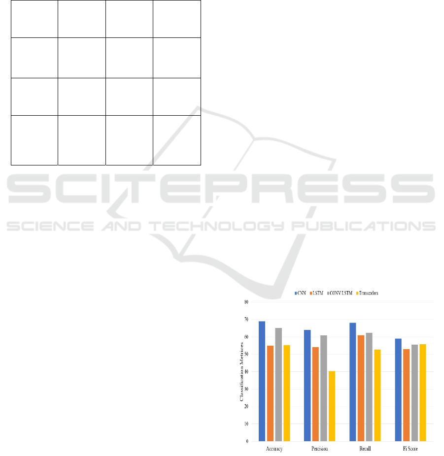
6.1 Classification Measurements

6.1.1 Confusion Matrix

Table 2: Correct and Inaccurate Predictions.

Predicted

Algae A

Predicted

Algae B

Predicted

Algae C

Actual

Algae A

20 (TP) 5 (FN) 1 (FN)

Actual

Algae B

3 (FP) 15 (TP) 2 (FN)

Actual

Algae C

0 (FP) 2 (FP) 18 (TP)

Table 2 displaying below is divided down by each

class, the number of correct and inaccurate

predictions given by a classifier. The figure 7 shows

Classification Metrics.

• True Positive (TP): Specific class

anticipated accurately.

• False Positive (FP): Said to be a specific

class but in reality, it belongs to another class.

• False Negative (FN): is not anticipated as a

given class while it truly belongs to that class.

• True Negative (TN): Designed to be not a

certain class, predicted precisely.

The model failed predicting Algae A five times (FN),

but accurately predicted Algae A twenty times (TP).

When Algae A was missing, the model

mistakenly predicted Algae A three times (FP).

By using these variables, one may create

accuracy, recall, and other metrics to analyze the

performance of the model for every class.

6.2 Accuracy

computes among all the model's predictions the

proportion of correct forecasts. The table 3 shows

Comparative study between Standard Technique and

Deep learning.

Acc(A) = sum of all estimated predictions/ Total no

of overall predictions

Here:

Correct guesses aggregated across all classes: 20 +

15 + 18 = 53.

Total number of predictions 53+5+3+1+2+2=66

Acc (A)= about 0.80.

6.3 Precision

Calculates among all the positive forecasts the

proportion of true positive predictions, sometimes

known as properly expected positives.

Precision (P) =TP/(TP+FP)

Precision (P for Algae A) = = 0.87 approximately.

Precision (P for Algae B) = = 0.75

Precision (P for Algae C) = ≈ 0.86

6.4 Recall

Calculates, from all the actual positives in the

dataset, the proportion of real positive predictions.

Recall (R for Algae A) =TP/(TP+FN)

Recall (R for Algae A) = 0.80 precisely.

Recall (R for Algae B) = = 0.88 approximately.

Recall (R for Algae C) = = 0.90 approximately.

6.5 F1-SCORE

Harmonic mean of accuracy and recall delivers a

reasonable evaluation of the two metrics.

F1 Score =2* (Precision*recall)/(Precision+Recall)

Algae A's F1 score Roughly 0.83

Algae B's F1 score equally 0.81

Algae C's F1 score Roughly 0.88

Figure 7: Classification Metrics.

ICRDICCT‘25 2025 - INTERNATIONAL CONFERENCE ON RESEARCH AND DEVELOPMENT IN INFORMATION,

COMMUNICATION, AND COMPUTING TECHNOLOGIES

122

Table 3: Comparative study between Standard Technique and Deep learning.

Categories Deep learning models Traditional models

Precision &

Predictive range

Usually displays outstanding accuracy when taught

on huge sets.

Can handle intricate interactions in the data and

nonlinear linkages.

Useful only on a tiny quantity of data. They

often may be tested against theoretical

frameworks and gives insights on causal

links.

Openness &

Interoperability

Though they are advancing in interpretability

methodologies, deep learning models may still

lack the direct causal insights afforded by

mechanistic models.

In ecological research, where verifying

model assumptions and grasping model

outputs hinges on enhanced interpretability

and transparency, classical methodologies

give precisely these traits.

Scalability &

Data

requirement

Although they are resource-intensive, deep

learning models gain from scalability with

enormous datasets.

Smaller datasets and preserve interpretability

make conventional techniques more

practical; consequently, they match studies

with constrained data availability or when

clear ecological theories lead modelling.

7 CONCLUSIONS

Marine environment prediction is a challenging task.

This work provides a detailed empirical analysis on

various deep learning algorithms used for

forecasting primary productivity in marine

environment. Various classification metrices were

also studied. Although deep learning models has

been applied successfully in various application

areas, building a appropriate model is essential

based on their variations and dynamic nature for the

real world problems. High level data representation

and large amount of raw data can be produced with

deep learning. A successful technique should provide

accurate data driven modelling based on the nature

of raw data. Deep learning has proved to be useful in

analysing various range of applications.

REFERENCES

Xu, L., Bennamoun, M., An, S., Sohel, F., & Boussaid, F.

(2019). Deep learning for marine species recognition.

In V. E. Bales, S. S. Roy, D. Sharma, & P. Samui

(Eds.), Handbook of Deep Learning Applications (pp.

129-145). (Smart Innovation, Systems and

Technologies; Vol. 136). Springer Science + Business

Media. https://doi.org/10.1007/978-3-030-11479-4_7.

Lumini, Alessandra & Nanni, Loris. (2019). Deep learning

and transfer learning features for plankton

classification. Ecological Informatics. 51.

10.1016/j.ecoinf.2019.02.007.

Bachimanchi, Harshith & Pinder, Matthew & Robert,

Chloé & De Wit, Pierre & Havenhand, Jon & Kinnby,

Alexandra & Midtvedt, Daniel & Selander, Erik &

Volpe, Giovanni. (2024). Deep‐learning‐powered data

analysis in plankton ecology. Limnology and

Oceanography Letters. 10.1002/lol2.10392.

Lopez-Vazquez, V., Lopez-Guede, J.M., Chatzievangelou,

D. et al. Deep learning based deep-sea automatic

image enhancement and animal species classification.

J Big Data 10, 37 (2023). https://doi.org/10.1186/s405

37-023-00711-w

D. Panzeri et al., "Defining a procedure for integrating

multiple oceanographic variables in ensemble models

of marine species distribution," 2021 International

Workshop on Metrology for the Sea; Learning to

Measure Sea Health Parameters (MetroSea), Reggio

Calabria, Italy, 2021, pp. 360-365, doi:

10.1109/MetroSea52177.2021.9611559.

Beery, Sara & Cole, Elijah & Parker, Joseph & Perona,

Pietro & Winner, Kevin. (2021). Species Distribution

Modeling for Machine Learning Practitioners: A

Review. 329-348. 10.1145/3460112.3471966.

Goodwin, Morten & Halvorsen, Kim & Jiao, Lei &

Knausgård, Kristian & Martin, Angela & Moyano,

Marta & Oomen, Rebekah & Rasmussen, Jeppe Have

& Sørdalen, Tonje & Thorbjørnsen, Susanna. (2022).

Unlocking the potential of deep learning for marine

ecology: Overview, applications, and outlook. ICES

Journal of Marine Science. 79. 10.1093/icesjms/fsab2

55.

Detection and Prediction of Primary Productivity in Coastal Environment Using Ensemble Models

123

Deivasigamani, Menaka & Gauni, Sabitha. (2021).

Parametric prediction of Ocean using Deep Learning

Technique for Sustainable Marine Environment. IEEE

Access. PP. 1-1. 10.1109/ACCESS.2021.3122237.

Marin, Ivana & Mladenovic, Sasa & Gotovac, Sven &

Zaharija, Goran. (2021). Deep-Feature-Based

Approach to Marine Debris Classification. Applied

Sciences. 11. 5644. 10.3390/app11125644.

Botella, Christophe & Joly, Alexis & Bonnet, Pierre &

Monestiez, Pascal & Munoz, François. (2018). A deep

learning approach to Species Distribution Modelling.

Alghazo, Jaafar & Bashar, Abul & Latif, Ghazanfar &

Zikria, Mohammed. (2021). Maritime Ship Detection

using Convolutional Neural Networks from Satellite

Images. 432-437. 10.1109/CSNT51715.2021.9509628.

Sasi, J.Priscilla & Pandagre, Karuna & Royappa, Angelina

& Walke, Suchita & G, Pavithra & L, Natrayan.

(2023). Deep Learning Techniques for Autonomous

Navigation of Underwater Robots. 1630-

1635.10.1109/UPCON59197.2023.10434865.

https://earthobservatory.nasa.gov/features/MeasuringVeget

ation/measuring_vegetation_2.php

Balasubramaniam J, Prasath D, Jayaraj KA.

Microphytobenthic biomass, species composition and

environmental gradients in the mangrove intertidal

region of the Andaman Archipelago, India. Environ

Monit Assess. 2017 May;189(5):231. doi:

10.1007/s10661-017-5936-0. Epub 2017 Apr 24.

PMID: 28439805.

S. F. Hagh et al., "Autonomous UAV-Mounted LoRaWAN

System for Real-Time Monitoring of Harmful Algal

Blooms (HABs) and Water Quality," in IEEE Sensors

Journal, vol. 24, no. 7, pp. 11414-11424, 1 April1,

2024, doi: 10.1109/JSEN.2024.3364142.

Y. Zhang, R. Ma, H. Duan, S. A. Loiselle, J. Xu and M.

Ma, "A Novel Algorithm to Estimate Algal Bloom

Coverage to Subpixel Resolution in Lake Taihu," in

IEEE Journal of Selected Topics in Applied Earth

Observations and Remote Sensing, vol. 7, no. 7, pp.

3060 3068, July 2014, doi:10.1109/JSTARS.2014.232

7076.

C. W. Park, J. J. Jeon, Y. H. Moon and I. K. Eom, "Single

Image Based Algal Bloom Detection Using Water

Body Extraction and Probabilistic Algae Indices," in

IEEE Access, vol. 7, pp. 84468-84478, 2019, doi:

10.1109/ACCESS.2019.2924660.

D. Xu, Y. Pu, M. Zhu, Z. Luan and K. Shi, "Automatic

Detection of Algal Blooms Using Sentinel-2 MSI and

Landsat OLI Images," in IEEE Journal of Selected

Topics in Applied Earth Observations and Remote

Sensing, vol. 14, pp. 8497-8511, 2021, doi:

10.1109/JSTARS.2021.3105746.

ICRDICCT‘25 2025 - INTERNATIONAL CONFERENCE ON RESEARCH AND DEVELOPMENT IN INFORMATION,

COMMUNICATION, AND COMPUTING TECHNOLOGIES

124