Enhancing Optical Sensor Image Classification through Deep

Learning with Convolutional Neural Network

S. Kumarganesh

, A. Gopalakrishnan

, B. Ragavendran

, S. Loganathan

, M. Gomathi

and I. Rajesh

Department of Electronics and Communication Engineering, Knowledge Institute of Technology,

Salem 637504, Tamil Nadu, India

Department of Artificial Intelligence and Data Science, Knowledge Institute of Technology,

Salem 637504, Tamil Nadu, India

Department of Information Technology, Muthayammal Polytechnic college, Rasipuram‑637408, Tamil Nadu, India

Department of Electronics and Communication Engineering, Paavai Engineering College,

Namakkal - 637 018, Tamil Nadu, India

Department of Information Technology, Vivekanandha College of Technology for Women,

Namakkal 637205, Tamil Nadu, India

Department of Computer Science and Engineering, Knowledge Institute of Technology, Salem 637504, Tamil Nadu, India

Keywords: Convolutional Neural Network (CNN), Optical Sensor (OS), Image Classification (IC), Deep Learning (DL),

Transfer Learning (TL).

Abstract: Applications for satellite images are numerous and include environmental surveillance, security, and disaster

recovery. Identifying infrastructure and entities in the images by hand is necessary for these applications.

Automation is necessary since there are numerous regions to be addressed and a limited number of specialists

accessible for performing the searches. However, the issue cannot be resolved by conventional object

recognition and categorization techniques since they are too erroneous and unstable. A set of machine learning

techniques called deep learning has demonstrated potential for automating these kinds of operations. Through

the use of convolutional neural networks, it proved effective at comprehending images. This paper

investigates how deep learning can be used to improve the categorization of optical sensor images, with an

emphasis on Convolutional Neural Network (CNN). Optical sensor pictures provide insightful information

for a variety of uses, including precision farming, tracking the environment, and analysis of land cover.

Consequently, to enable more precise and effective categorization, this research makes use of CNN ability to

automatically develop hierarchical representations. The effectiveness of deep learning within this field is

demonstrated by comparing the model's performance versus conventional classification techniques. The

results of this study add to the expanding amount of research in remote sensing utilizing image analysis by

offering a solid framework for enhancing the precision and effectiveness of optical sensor picture

categorization by utilizing CNN and innovative deep-learning methods. MATLAB is used to implement the

suggested framework. The suggested approach outperformed region-based GeneSIS, OBIA, segmentation

and classification tree method, fuzzy C means, and segmentation with an accuracy of 95%.

1 INTRODUCTION

Optical sensor images are essential to modern remote

sensing because they collect visible and near-infrared

wavelengths, providing a unique view of the Earth's

surface. Sensors like this are essential parts of

satellites as well as other aerial platforms, offering a

large amount of data for a wide range of uses, such as

agricultural management, environmental surveillance,

hazard review, and land use classification. Optical

sensors work fundamentally by identifying and

capturing sunlight scattered off the surface of the

Earth. Different surface characteristics may be

distinguished due to the sensors' numerous spectral

bands, which each catch light at a distinct wavelength

(C. Li et al., 2019). In addition to the near-infrared,

which can be especially useful for vegetative study,

typical spectral categories include the red, green, and

blue bands. High spatial resolution optical sensor

pictures deliver comprehensive images of the surface

of the Earth, which is one of their main advantages.

676

Kumarganesh, S., Gopalakrishnan, A., Ragavendran, B., Loganathan, S., Gomathi, M. and Rajesh, I.

Enhancing Optical Sensor Image Classiﬁcation through Deep Learning with Convolutional Neural Network.

DOI: 10.5220/0013888400004919

Paper published under CC license (CC BY-NC-ND 4.0)

In Proceedings of the 1st International Conference on Research and Development in Information, Communication, and Computing Technologies (ICRDICCT‘25 2025) - Volume 2, pages

676-691

ISBN: 978-989-758-777-1

This quality is critical for activities where precise

decision-making depends on tiny details, like

precision farming, urban design, and tracking

infrastructure. Optical sensor images greatly enhance

environmental surveillance. These sensors can track

urbanization, recognize deforestation, identify

variations in land cover, and evaluate ecosystem

health. Moreover, optical pictures play a crucial role

in the research of natural catastrophes, supporting the

evaluation of the damage resulting from crises like

earthquakes, floods, as well as wildfires (B. Rasti and

P. Chamise 2020)

Optical sensor pictures help with precision

farming in agriculture by revealing information about

the health of crops and the vitality of plant life.

Farmers can enhance water supply, by applying

fertilizers, and insect management by being able to

discern among affected and healthy vegetation due to

the distinct spectrum. This accuracy supports

sustainable farming methods and higher crop yields.

Optical sensor image incorporation with geographic

information systems (GIS) makes it easier to create

precise and comprehensive maps. Optical imagery-

derived maps of land use and vegetation are important

tools for managing resources, urban development, and

preservation of the environment. A fundamental

component of remote sensing, optical sensor images

provide for a thorough comprehension of the motions

in the Earth's surface (Y. Bazi et al., 2021). They have

a wide range of uses and offer vital data for disaster,

farming, and environmental control. The combination

of sophisticated analytical methods like deep learning

with optical sensor imaging has an opportunity to

significantly improve the capacity to observe and

understand the complexity of this developing planet as

technology develops.

A vital component of remote sensing as well as

geospatial analysis is the classification of optical

sensor images, which uses innovative methods to

analyse and classify data gathered from optical sensor

imaging. Through this method, different areas or

pixels inside a picture are assigned specific groups or

signs, enabling a detailed comprehension of the

exterior of the Earth and its changing aspects. The

fundamental goal in optical sensor image

categorization is to automatically extract useful data

from enormous data sets so that it may be used for

effective evaluation and selection in a variety of fields.

Applications including land cover visualization,

agriculture, urban development, environmental

monitoring, and disaster response fall under this

category. Advanced categorization algorithms

transform optical sensor images into indispensable

instruments for deriving meaningful conclusions from

detailed visual data (M. P. Uddin et al., 2021). The

initial phase in the categorization process is obtaining

excellent quality optical sensor imagery, which is

usually obtained using satellites or aerial platforms.

There are several spectral bands in these pictures, and

each one corresponds to a distinct light wavelength.

Typical bands that together give a complete picture of

the Earth's surface are red, green, and blue, along with

near-infrared. Categorization is based on the unique

spectral fingerprints of different features, including

flora, water, cities, and bare soil. Usually obtained by

satellites or aerial platforms, the categorization

process starts with the collection of detailed optical

sensor imagery. Several spectral bands, each denoting

a distinct light wavelength, are seen in these pictures.

Red, green, blue, as well as near-infrared are common

bands that together offer a complete picture of the

surface of the earth. Categorization is based on the

different spectral signatures of different

characteristics, including bare soil, vegetation, water,

and urban surroundings (F. Zhou and Y. Chai et al.,

2020).

The two main methods used in visual sensor

classification of images are supervised as well as

unsupervised classification. A machine learning

algorithm is developed utilizing labelled samples,

wherever each pixel in the image is connected with an

identified class, in supervised classification. The

remaining pixels are subsequently classified using

machine learning methods, such as random forests,

neural networks, and support vector machines, among

others, by the patterns that were previously learned

(X. Lei, H. Pan, and X. Huang et al., 2019). In contrast,

unsupervised classification entails clustering pixels

without the need for pre-established classifications.

To find patterns and groups, this approach depends on

the data's intrinsic statistical characteristics. In

unsupervised classification, clustering algorithms like

k-means as well as hierarchical clustering are

frequently utilized. Optical sensor image

categorization has several issues, such as managing

environmental conditions, spectral fluctuation, and

mixed pixels a pixel that combines information from

several types of land cover. Processing techniques like

atmospheric and radiometric adjustments are

frequently used to lessen these difficulties and

improve the precision of the categorization findings.

The inclusion of deep learning methods, in particular,

Convolutional Neural Networks has greatly improved

the categorization of optical sensor images. To capture

complex patterns including spatial connections, CNNs

are particularly good at developing hierarchical

features from images. Deep learning-based

classification techniques become even more accurate

Enhancing Optical Sensor Image Classiﬁcation through Deep Learning with Convolutional Neural Network

677

and efficient via transfer learning, in which trained

models are adjusted for particular classification tasks

(S. Bera and V. K. Shrivastava 2020).

More and more high-resolution optical sensor

footage is becoming available, opening up previously

unheard-of possibilities for monitoring the

environment, land cover mapping, and earth

observations. The abundance of data obtained by

optical sensors offers a valuable resource for resource

management and knowledge on planet. However, the

real use of this imagery depends on precise and

successful classification algorithms that can identify

intricate patterns and characteristics in the data. The

fine features present in high-resolution optical sensor

images frequently make conventional image

categorization techniques ineffective. This work sets

out to improve optical sensor image classification by

employing deep learning, with a particular emphasis

on CNNs, as a solution to these difficulties (L. Khelifi

and M. Mignotte 2020). In the field of image analysis,

deep learning has become a game-changing paradigm

that has shown amazing promise across a range of

applications, including computer vision, healthcare

imaging, and remote sensing. An especially good

subclass of deep learning algorithms for

autonomously extracting structured representations

from picture data is CNNs. They are particularly well-

suited for jobs like optical sensor image classification,

where minute details are essential for precise

interpretation, because of their capacity to record

complex spatial data. The realization that using CNNs

to their full potential will greatly increase the precision

and effectiveness of optical sensor image

classification is what spurred this research.

Customized feature extraction, which is typical in

traditional picture classification algorithms, has

limitations. Deep learning mitigates these limitations

by enabling the algorithm to learn its own useful

features from the data (Y. Feng et al., 2019).

The pre-processing of optical sensor data is the

first step in the extensive pipeline that makes up the

methodology used in this work. The model is trained

with normalization and augmentation techniques to

improve its ability to generalize patterns in a variety

of settings and conditions. Afterward, a meticulously

selected dataset is utilized for both assessment and

training, guaranteeing that the model is exposed to a

typical portion of optical sensor imagery (D. Hong et

al., 2020). The proposed methodology is based on the

creation of a CNN framework specifically engineered

for the classification of images from optical sensors.

Because the CNN is set up to extract features

hierarchically, the model can identify global as well as

local trends in the picture. Thorough experimentation

is used to validate the architecture's efficacy and

recognized measures like accuracy, precision, recall,

and F1-score are used to assess the model's

performance. This study investigates the possibilities

of transfer learning as well as fine-tuning approaches,

going beyond the traditional bounds of deep learning.

The research focuses in particular on the use of the

ResNet50 design, a deep neural network that has

already been trained, for optical sensor image

classification. Transfer learning is a technique that

improves performance on one job (like image

recognition) by utilizing knowledge from another

related task (like optical sensor image classification).

The model that was previously trained is further

improved by fine-tuning so that it can conform to the

unique subtleties of the optical sensor images. In brief,

this study attempts to advance the development of

methods for classifying optical sensor images by

utilizing CNN's powers inside a structure for deep

learning. The ensuing sections of this research will

examine the comprehensive technique, experimental

outcomes, and conversations that jointly mould the

comprehension of the possibilities and obstacles

linked with this innovative strategy. The following are

the main contributions:

• CNNs are utilized to automatically extract

hierarchical characteristics from optical

sensor images, thereby capturing

complicated patterns and spatial correlations

for improved classification accuracy.

• By combining deep learning techniques with

CNNs, the model's capacity to generalize

patterns over many scenarios and

environments is improved, leading to better

classification results on unknown data in a

variety of environmental contexts.

• This method, which uses CNNs, lessens the

dependence on features that are manually

generated, enabling the model to

independently learn and adjust to the

distinctive qualities seen in optical sensor

pictures.

• CNNs are particularly good at analysing

high-resolution optical sensor pictures

because they can handle the extensive details

included in the data and offer a solid

foundation for accurate land cover

classification.

• By utilizing information from larger image

data sets, transfer learning techniques more

specifically, fine-tuning pre-trained CNN

models help to increase classification

precision and effectiveness in optical sensor

image processing.

ICRDICCT‘25 2025 - INTERNATIONAL CONFERENCE ON RESEARCH AND DEVELOPMENT IN INFORMATION,

COMMUNICATION, AND COMPUTING TECHNOLOGIES

678

To allow for an organized investigation of the

subject, this work is divided into multiple important

sections. Section 1 provides background details and

explains how and why using CNNs in conjunction

with deep learning can enhance the classification of

optical sensor images. Section 2 outlines the

procedures for initial processing, preparing the data,

and CNN structure in addition to the related works

approach. Section 3 describes the limitations of the

current system. In Section 4, the suggested framework

methodology is explained. Section 5 presents the

experimental results and evaluates the model's

performance using standard metrics. Section 6, which

provides guidance for future research and highlights

significant findings, serves as the work's final section.

2 RELATED WORKS

Deep learning-based techniques for classifying

hyperspectral images (HSI) have advanced

significantly in the last few years. The accuracy of

classification is significantly enhanced by these data-

driven approaches' improved feature extraction

capabilities. Nevertheless, to achieve the ability to

extract features adaptable for the target picture when

confronted with a fresh HSI for classification, the

prior methods typically necessitate retraining the

networks from the start, which is a laborious and

repetitive procedure. Sun et al. 2022. Think about

delaying this procedure and using pre-training to give

the network strong feature extraction and

generalization capabilities. As a result, without the

need for retraining, the network allows for the

immediate extraction of specific HSI properties. In

order to do this, they reconsider the 3-D HSI data

collected from the standpoint of spectroscopic

sequence and make an effort to extract information

about spectral variations as the spectrum's movement

characteristic. Then, to learn the information about

detecting spectral variations, they build an

unsupervised spectrum movement feature learning

structure (SMF-UL) that can be trained on bulk

unstructured HSI data. Additionally, create an

expandable training dataset to accomplish the

enlargement of the original information for initial

training. A construction approach that may efficiently

use the constantly expanding bulk of unlabelled HSI

data by integrating sensors, bands, and HSIs of

various sizes into a single training set. Lastly,

to prevent the tedious process of retraining the

network, they employ the network that was trained to

immediately gather the spectrum of motion

characteristic of the desired HSI for classification.

Numerous tests demonstrate that the suggested SMF-

UL gains the reliable ability to extract features with

generalization through unsupervised training on large

amounts of unlabelled HSI data. Additionally, the

obtained spectrum motion feature's accuracy in

classification is comparable to sophisticated in-

domain and cross-domain techniques, demonstrating

its flexibility and supremacy.

Xu et al.,2019 presents the scientific results of the

IEEE Geophysical and Remote Sensing (RS)

Society's Image Processing and Data Fusing

Technical Committee's 2018 Data Fusion Contest.

Using sophisticated multi-source optical remote

sensing techniques (multispectral LiDAR,

hyperspectral photographic imaging, and very

excellent quality imagery), the 2018 Competition

tackled the topic of urban surveillance and

supervision. The goal of the competition was to

differentiate between a wide range of intricate

classifications of urban items, materials, and

vegetation based on the classification of the use of

urban land and land cover. In addition to merging

data, it measured the individual strengths of the new

sensors that were employed to get the information. To

maximise the amount of data accessible, participants

suggested complex strategies based on machine

learning, computer vision, and remote sensing. It's

also important to note that post-processing and ad hoc

classifiers were crucial in both winner records,

contributing to a 15% improvement in total accuracy.

Even though decision fusion techniques were

previously presented in this study, there is still more

work to be completed, particularly in terms of

automatically integrating and fusing expert

information into NNs. Furthermore, this kind of

knowledge typically makes sense for all individuals

and supports the choice. It will be lucrative to do more

study to make CNN more understandable to aid in the

public's acceptance and spread of these techniques. In

terms of the information, multi-spectral LiDAR by

itself and even the fusion of various sources was

shown to be very insightful, as these sensors yielded

the best LULC categories (accuracies of over 80% in

general and 71% on average). Additionally, rasterized

2.5D was the sole method used to handle LiDAR data.

This points to possible directions for creating

methods that can analyse and categorize actual 3-D

sensor data. The data was re-released after the

competition and will continue to be freely accessible

for the society's advantage. All relevant material is

available on the IEEE GRSS site for

anyone interested. The training data with matching

labels or the test information can be downloaded after

enrolling on the IEEE GRSS DASE server. The

Enhancing Optical Sensor Image Classiﬁcation through Deep Learning with Convolutional Neural Network

679

classification outcomes can then be submitted to

receive efficiency statistics, compared with other

customers, and, ideally, improve upon the results

reported in this work. Because it is the biggest

accessible HS dataset having ten times more labelled

data compared to the popular Salinas or Pavia

datasets or the initial multispectral-LiDAR dataset,

we do think it could have a significant influence on

the integration of data study as well as the growth of

single-sensor handling.

Li et al.,2019 explains that the classification of

ground objects paired with multivariable optical

sensors is an important subject at the moment because

of the advent of high-resolution optical sensors.

Convolutional neural networks and other deep

learning techniques are used for feature extraction

and categorization. This paper proposes a unique

hyperspectral image classification technique using

deep belief networks (DBNs) stacked by limited

Boltzmann machines and multimodal optical sensors.

To categorize spatially hyperspectral data collected

by sensors using DBN. Subsequently, the enhanced

approach which combined spectral and geographical

data was confirmed. The DBN model was able to

acquire features after supervision fine-tuning and

uncontrolled pre training. They also included logistic

regression layers so that the hyperspectral photos

could be categorized. Additionally, tests were

conducted using the Indian Pines and Pavia

Universities dataset to evaluate the suggested training

strategy, which combines spectral and spatial data.

The following are the benefits of this approach over

conventional methods: Tests show that the method

beats other deep learning algorithms and

conventional classification. (1) The neural network

has a complex structure and a higher ability to gather

features than conventional classifiers. Features

impact the final model's performance and serve as its

training information. In theory, a deep neural network

(DNN) could gather more information and learn more

complicated functions if it has additional concealed

layers. Consequently, a detailed description of the

DNN model is possible. Based on the DBN approach,

this paper suggests a novel approach to hyperspectral

picture classification. Pre training, modification, and

data pre-processing are all part of the fundamental

DBN classification paradigm. The incorporation of

pre training distinguishes DBN from a neural

network. In the DBN model, the starting weight value

may be rather near to the global optimization.

Consequently, the accuracy of the greedy layer-wise

supervision learning is higher than that of a neural

network. The mini-batch DBN model verifies the

learned characteristics and the loss functions to

update the weights w during the supervised fine-

tuning process. During every training period,

variables are taught in mini-batches.

Popowicz and Farah 2020, explores the complex

field of dark current, which is a crucial component

that affects the appearance of scientific photographs

that are obtained using charge-coupled devices

(CCDs). Impulsive noise in pictures is frequently

caused by dark current, which is a result of faults and

contaminants in the fabrication process. Its stability

has historically been associated with temperature. But

the study also reveals a unique feature of dark

currents in proton-irradiated detectors: a range

of metastable phases that present formidable

obstacles to picture correction. Using Kodak KAI

11000M CCD sensors, which were used for seven

years of in-orbit operations during the BRITE

(Brightest Target Explorer) astrophysics mission, the

study covers a hitherto unheard-of temporal range,

wide temperature changes, and a large number of

examined pixels. An essential tool for locating and

describing these metastable phases in the dark current

is a specialized methodology based on the Gaussian

mixture model. The results give a sophisticated

understanding of the features of the Meta stabilities

linked to dark current and provide significant fresh

insights into how they operate. The study provides

new insights into the difficulties of modelling and

controlling dark currents in image sensors used in a

challenging space environment. Specifically, the

study reveals experimental laws guiding the

behaviour of darkness current in tri stable faults. This

provides a thorough examination, opening the door to

better methods for calibrating and enhancing the

performance of image sensors, especially in the

setting of astrophysics expeditions where accurate

and trustworthy image data is crucial. This study

addresses important features of image sensor

operation in space applications, and its long duration

and thorough investigation of dark current features

make it a substantial contribution to the area.

Labelling land use/land cover (LULC) gathered

by several sensors with varying spectral,

geographical, and temporal resolution is facilitated by

the use of remote sensing data. For the investigation

of LULC change and modelling in hazy mountain

regions, the combination of an optical image with a

synthetic apertures radar (SAR) image is important.

Zhang et al. 2020 proposes a unique feature-level

fusion framework, wherein LULC classification

experiments are carried out using a fully polarised

Advanced Land Observing Satellite-2 (ALOS-2)

picture and Landsat operational land imager (OLI)

images that have different cloud coverings. They use

ICRDICCT‘25 2025 - INTERNATIONAL CONFERENCE ON RESEARCH AND DEVELOPMENT IN INFORMATION,

COMMUNICATION, AND COMPUTING TECHNOLOGIES

680

the Karst Mountains in Chengdu as study region.

After that, they extract the characteristics from the

optical and SAR pictures' spectrum, texture, and

space, correspondingly. They also add additional

pertinent data, such as altitude, slope, and the

normalized difference vegetation index (NDVI).

Moreover, object-oriented multi-scale segmentation

is applied to the fusion features image, and the study

is then carried out using an enhanced SVM models.

The outcomes demonstrated the benefits of the

suggested framework, which include high

classification efficiency, data from multiple sources,

a combination of features, and use in mountainous

regions. Overall accuracy (OA) was over 85%, and

the values of the Kappa coefficient were 0.845. When

it came to artificial surfaces, lakes, gardens, and

forests, the fusion image's accuracy was greater than

that of a single source of information. Furthermore,

there is a relative benefit in the collection of water,

artificial surfaces, and shrub land using ALOS-2 data.

The purpose of this study is to serve as a guide for

choosing appropriate data and techniques for LULC

categorization in misty mountain regions. In overcast

mountainous regions, the fusion characteristics of the

pictures should be prioritized; in less cloudy periods,

Landsat OLI data must be chosen; and in situations

where data from optical remote sensing are

unavailable, fully polarised ALOS-2 data are a

suitable stand-in.

In general, this collection of research papers

covers a broad range of topics in the field of remote

sensing and highlights advancements in classification

methods and applications. To create strong extracting

feature capabilities without requiring a lot of

retraining, a method for unattended spectrum motion

learning of features in hyperspectral image

classification. An enhanced multi-sensor optical

imaging for urbanized land cover and land use

categorization is discussed along with the results of

the 2018 IEEE GRSS Information Fusion

Competition. It emphasizes how different optical

sensors can be integrated and how convolutional

neural networks function well for addressing intricate

and varied urban classes. The benefits of deep

learning over conventional techniques for feature

extraction and classification, proposing a deep belief

network methodology for spectral-spatial grouping of

hyperspectral distant sensor data. The metastable dark

currents in BRITE Nano-satellite imaging sensors

provides a thorough examination of the metastable in

nature states in charge-coupled electronics and their

consequences for astrophysics missions' image

calibrating. To enhance classification performance

via multi-source data integration, an innovative

feature-level fusion framework for classifying land

use and land cover in overcast mountainous locations

using optically and SAR sensor pictures.

Nevertheless, these studies have certain drawbacks,

such as the requirement for large labelled datasets, the

influence of metastable dark currents on image

resolution in space-based detectors, and possible

difficulties in interpreting the models for deep

learning techniques (B, Selvalakshmi, Hemalatha K,

et al. 2025). Additional investigation could

potentially tackle these constraints and improve the

usefulness of the suggested approaches.

3 PROBLEM STATEMENT

The current optical sensor image classification

algorithms have several drawbacks, including the use

of handmade characteristics that may not be able to

adequately capture the complex patterns found in

high-resolution imaging. The intricacy and

unpredictability of optical sensor information can

pose challenges to traditional approaches, particularly

in situations where there are a variety of land cover

types (L. Ding, H. Tang, and L. Bruzzone 2020).

Significant obstacles also include the requirement for

laborious manual tagging and the difficulty of

generalizing to previously unseen data. However,

there are strong benefits to using CNN and deep

learning for optical sensor picture classification. The

model is able to identify intricate spatial connections

and trends within optical sensor pictures thanks to the

use of deep learning with CNNs that enables

automated (P, Elayaraja et al., 2024) and hierarchy

extraction of features. By enhancing the algorithm's

flexibility to various scenarios and drastically

reducing reliance on manually created features, this

technology eventually improves classification

effectiveness and precision. Additionally, the

application of CNNs facilitates transfer learning by

enabling the algorithm to be customised for particular

optical sensor datasets and take advantage of

information from pre-trained networks, hence

resolving the issues related to the requirement for

huge labelled datasets. In general, the deep learning-

based method improves optical sensor image

classification's durability, accuracy, and

generalization capabilities, which makes it an

exciting advance for remote sensing uses.

Enhancing Optical Sensor Image Classiﬁcation through Deep Learning with Convolutional Neural Network

681

4 OPTICAL SENSOR IMAGE

CLASSIFICATION THROUGH

DEEP LEARNING WITH

CONVOLUTIONAL NEURAL

NETWORK

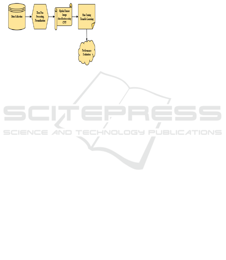
Figure 1: Architecture diagram of proposed CNN transfer

learning model.

Several crucial phases are included in the process

for improving the optical sensor classification of

images using deep learning with CNNs. Initially, pre-

processing is applied to the optical sensor imagery,

including activities like normalization to improve a

model's generalisation across various settings and

conditions. After that, a large dataset is carefully

selected to guarantee that a variety of optical sensor

images are represented for training and assessment.

Next, the convolutional and pooling phases of the

CNN architecture are set up and tailored to support

the hierarchical extraction of features, thereby

preserving spatial patterns and correlations. During

the training stage, backpropagation and optimization

methods are used to adjust the CNN's weights using

the carefully selected dataset. By using CNN models

that have been trained on extensive image datasets,

transfer learning is investigated to improve the

model's ability to extract features. Validation datasets

are used, and hyper parameters are adjusted,

to reduce excessive fitting. After training, the CNN is

used to classify previously unknown optical sensor

images, and its efficacy is carefully assessed using

common metrics such as accuracy, precision, recall,

and F1-score. The whole approach seeks to improve

the precision and effectiveness of land cover

categorization by utilizing deep learning to learn on

its own and retrieve characteristics from optical

sensor data.

Figure 1 illustrates the methodical procedure that

deep learning using CNNs uses to improve optical

sensor image classification. To improve the model's

resilience, raw optical sensor pictures are first pre-

processed and then normalized and enhanced. Then,

appropriate samples for training and evaluation are

included in a diversified dataset. Convolutional and

pooling layers are included in the design of CNN to

enable hierarchical feature extraction. To maximize

the model's adaptation to optical sensor input, transfer

learning is used by initializing the framework with

weights that have been trained. During the training

stage, the CNN is fed the carefully selected dataset,

and optimization and backpropagation methods are

used to adjust the model's parameters. In order to

avoid overfitting, validation data sets are useful for

hyper parameter tweaking. Following training,

unknown optical sensor image classification is

carried out by CNN, and standard metrics are

employed to thoroughly assess the accuracy of the

model. By utilizing the capabilities of deep learning,

this method greatly increases the precision and

effectiveness of land cover categorization by

enabling CNN to independently learn complicated

characteristics from optical sensor data.

4.1 Data Collection

The suggested feature-selection strategy is evaluated

using the RSSCN7.2 sensor scenario data set (Z. Zhao

et al., 2020). Sensor images from three distinct groups

make up the data collection RSSCN7. The datasets

have been designated as follows: Water, Land, and

Forest. A total of 400 images were gathered from

Google Earth for every group; these images have

been selected on four distinct scales, with 100 images

for every level. Every picture is 400 x 400 pixels in

size. Because of the extensive variety of scene photos

that are collected on various scales and taken in a

range of weather conditions and seasons, this

gathering of information presents certain difficulties.

There is a set of training as well as validation data sets

built for every optical sensor image.

4.2 Data Pre-Processing

To standardize the size of input characteristics and

guarantee consistent and accurate model training,

data normalization is a crucial pre-processing

technique that is frequently used in machine learning

as well as deep learning. The principal aim is to

convert numerical information into a uniform range,

mitigating the effects of disparate scales and fostering

convergence in the training stage. Data normalization

in the setting of optical sensor image classification

with CNNs entails modifying the picture pixel

values. Scaling the value of pixels to a conventional

ICRDICCT‘25 2025 - INTERNATIONAL CONFERENCE ON RESEARCH AND DEVELOPMENT IN INFORMATION,

COMMUNICATION, AND COMPUTING TECHNOLOGIES

682

range, like [0, 1] or [-1, 1], is a popular method. This

is commonly accomplished by deducting the average

pixel intensity value and dividing the result by the

standard deviation. Normalization prevents some

characteristics from predominating because of

disparities in magnitude by ensuring every feature

(pixel) serves proportionately to the model's learning

process. This procedure improves the model's

capacity to identify correlations and trends in the

optical sensor visuals, which in turn improves

classification accuracy and generalization. It also

helps the system converge more quickly throughout

training.

A statistical method called data normalization is

used for scaling and centring a feature's

measurements to ensure they lie in a predetermined

range. Normalization is carried out to the picture

values of pixels in the setting of classifying optical

sensor images using CNNs. The typical normalization

formula is shown in eqn. (1):

𝑁=





(1)

Where E is the data sets mean, SD is the Standard

Deviation, and j is the variable's starting value.

Deviation Z is the standardized value.

The data is scaled to have a variance of one and is

centred on zero throughout the normalization

procedure. By ensuring that the characteristics have

comparable scales, this change stops some features

from controlling the learning process because of

disparities in size. For deep learning algorithms, such

as CNNs, to be trained effectively, optimization

methods, such as that of gradient descent, must

converge. Normalization helps the model perform

better and converge more quickly on optical sensor

imagery, which improves model generalization.

4.3 Convolutional Neural Network

A CNN is a particular kind of deep neural network

that is used to handle data that resembles a grid,

including frames from videos and photos. In the field

of optical sensor image classification, CNNs are

essential because they offer a strong framework for

identifying complicated patterns and characteristics

in the images. CNNs use convolutional layers in

optical sensor classification to identify unique visual

features like edges, colours, and spatial patterns.

Activation functions for adding non-linearity, such as

Rectified Linear Unit (ReLU), pooling layers for

spatial down sampling, and fully linked layers for the

highest-level feature integration, come after these

layers. The CNN architecture is especially

appropriate to the subtleties of optical sensor data

because it makes it possible for structured

representations to be automatically learned. This is

key for distinguishing minute details that are

important for classifying land cover and land use.

Moreover, transfer learning in which CNNs use

models that have been trained on massive image

datasets works well in situations where there is a

dearth of labelled optical sensor data because it

enables the model to adjust and perform well in

particular optical sensor tasks such as classification.

In addition to improving classification accuracy, the

combination of CNNs and optical sensor data offers a

strong basis for deriving significant insights from a

variety of dynamical optical sensor pictures.

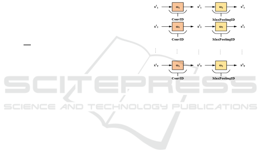
Figure 2: CNN Architecture.

Convolutional, pooling, and fully linked layers

are among the layers that make up CNN. Figure 2.

displays the CNN architectural diagram.

4.3.1 Input Layer

Typically, a CNN receives a picture as input in the

form of an ordered set of pixel values. The physical

dimensions of an image (e.g., 224 x 224 pixels for an

ordinary image classification assignment) dictate the

size of the input.

4.3.2 Convolutional Layer

The layer having the most powerful signature in a

CNN is the convolutional layer, which is the first step

in the extraction of features. The extraction of various

contours from the input sensor images is the local

operation's purpose, which results in an efficient

classification. Convolutional layers consist of

several convolutional kernels, which are the trainable

parameters that vary with every iteration of the layer

is shown in eqn. (2).

Enhancing Optical Sensor Image Classiﬁcation through Deep Learning with Convolutional Neural Network

683

𝑆

(

𝑖,𝑗

)

(

𝐼∗𝐾

)(

𝑖,𝑗

)

= ∑



∑



𝐼

(

𝑖+𝑚,𝑗+𝑛

)

⋅𝐾(𝑚,𝑛)

(2)

𝑆

(

𝑖,𝑗

)

represents the output of the convolution

procedure at point

(

𝑖,𝑗

)

in the resultant feature map.

I am a representation of the input matrix, which

is typically a feature map or picture. The symbol K

represents the convolution kernel. ∑



and ∑



indicate the total of the spatial dimensions of the

kernel. The symbol

(

𝑖+𝑚,𝑗+𝑛

)

represents the

pixel value of the input matrix at location𝐼(𝑖 + 𝑚,𝑗 +

𝑛). 𝐾(𝑚,𝑛) represents the quantity (or filter

coefficient) inside the convolution kernels at position

(𝑚,𝑛). CNNs usually have a large number of

convolutional layering in an attempt to identify more

distinct patterns of space in the input images. Keeping

the image sizes constant throughout the process is

ensured by employing zero padding in conjunction

with convolutional layers.

4.3.3 Pooling Layer

Let 𝐺





∈𝑅





×



×



be the input of the N-th layer,

which is essentially a layer for pooling that has a

longitudinal range of 𝑚′ × 𝑛’. These layers are

parameter-free since they don't have any variables

that need to be learned. They assume that m' divides

M, n' divides N, and stride matches the pooling

longitudinal span. The outcome is represented as

𝑌



∈𝑅





×



×



, which is a tensor of order

three given in eqn. (3),

𝑀









,𝑁









,𝐷



=𝐷



(3)

In contrast, each 𝐺





channel is handled separately

and one at a time by the pooling layer. Although there

are numerous distinct pooling techniques, the most

used ones are average and maximal pooling. When

max-pooling was used in the study, the outcomes

followed an eqn. (4):

𝑦





,



,

=𝐺





×∗∗,



×∗∗,



(4)

It seems natural that pooling layers could be used

to minimize output tensor size while maintaining the

most significant detected characteristics where

0≤

𝑖

∗

≤𝑀

∗

,0≤𝑗

∗

≤𝑁



and 0≤𝑑≤𝐷



4.3.4 Fully Connected Layer

This layer, referred to as another portion of the CNN,

functions by successfully sorting the features that

were obtained by the first component. The input of

the primary fully linked layer is a highly dimensional

vector that contains each feature that was extracted

and created as the outcome of a smoothing procedure.

After the last completely linked layer, a classification

operation (soft max, sigmoid, tanh, etc.) is always

applied. With the selected loss function, the actual

value 𝑦



is contrasted to the expected value𝑦



applying the sigmoid function in this case is given as

eqn. (5).

𝑦















, 𝐺



∈𝑅 (5)

Where, the output 𝐺



∈𝑅 is frequently utilized

in neural networks. This function is appropriate for

issues with binary classification since it converts an

input, 𝐺



, through a value that ranges from 0 to 1. 𝑒





is the term that is the increasing function, and 𝑒





the denominator, makes sure the result is a legitimate

probability. Based on the input 𝐺



, the result 𝑦



can be

interpreted as the probability of a binary event.

4.3.5 Rectified Linear Unit

Another crucial idea is dropout, a strategy for making

the learning process more universal while lowering

the possibility of overfitting. It brings back to zero the

configurations associated with a given number of

network nodes. Lastly, the processes of batch

normalisation and Rectified Linear Unit (ReLU)

function as essential transitory mechanisms

connecting the aforementioned stages. The ReLU

function's description is given in eqn. (6).

𝑦

,,

=0,𝐺

,,



 (6)

Batch regularisation increases the speed and

stability of neural networks by regularising the layer's

input by rescaling and re-centering it after each

iteration. It does this by trying to transfer only the

elements required for the classification using 0≤𝑖≤

𝑀^𝑛,0≤𝑗≤𝑁^𝑛,𝑎𝑛𝑑 0≧𝑑≤𝐷^𝑛.

4.3.6 SoftMax Layer

In Convolutional Neural Networks as well as other

neural network topologies, the SoftMax layer is an

essential component, particularly in classification

tasks. Since the output layer, is usually utilized to

convert the network's basic output values into

probability distributions across several classes. The

outcomes are guaranteed to be balanced and to

indicate probability by the SoftMax function. Eqn. (7)

provides the SoftMax layer formula.

𝑓𝑖 =







∑











(7)

The basic logarithm, or Euler's number, has a base

of u, and the initial score or logit for class a is

ICRDICCT‘25 2025 - INTERNATIONAL CONFERENCE ON RESEARCH AND DEVELOPMENT IN INFORMATION,

COMMUNICATION, AND COMPUTING TECHNOLOGIES

684

represented by 𝑎



∑

𝑢









represents the total

exponentiated logarithms for all classes.

4.4 Transfer Learning

Transfer learning in CNN representations has

demonstrated that CNN layers may be applied from

natural images to various medical data, including CT

(computed tomography) images, ultrasonic data, and

neuroimaging data, either by fine-tuning the settings

or by using the pre-made models. The term "transfer

learning" relates to a method of machine learning that

enables knowledge from one domain to be applied to

related domains and issues. It is advised to start a task

that is identical to the trained model by using the

model that was created and trained for that task. In

order to define transfer learning, researchers have

employed a variety of notations to explain its various

principles. The two fundamental ideas of transfer

learning are domain and task, both of which have

mathematical explanations. To help with clarity,

transfer learning is explained arithmetically. The two

components that makeup Domain M are the marginal

distribution H (G) and the feature space which is

shown in eqn. (8).

𝑀=𝑔,𝐻(𝐺) (8)

G is an occurrence set (also known as an instance

set) in this case, and it can be understood as 𝐺=

{𝑦|𝑦



∈𝑔,𝑗=1,..,𝑛} . Task T consists of a label

space L and a judgment function t of eqn. (9).

𝐴={𝐵,𝑎} (9)

Utilizing pre-trained models' expertise from

general image recognition tasks and tailoring it to the

particular job of optical sensor image classification is

known as transfer learning. This approach is used to

improve optical sensor image classifications through

deep learning with CNNs. To start, a CNN model that

has been previously trained is initialized. The pre-

trained model's convolutional layers function as

efficient feature extractors, identifying subtle and

intermediate visual patterns. The pre-trained model's

last layers are changed or replaced in the adaption

step to correspond with the number of categories in

optical sensor images. Next, fine-tuning is performed

on the newly created dataset of tagged optical sensor

images by minimizing the cross-entropy loss is given

in eqn. (10).

𝑂=(𝑥,𝑥)



=−(𝑥log

(

𝑥

)

(

1−𝑥

)

log (1 − 𝑥) (10)

Where x is the real label (0 or 1) and x ̂ is the

expected probability of a class that is positive. The

cross-entropy loss is used to quantify the difference

between the true labels of the fresh dataset and the

anticipated class likelihoods when fine-tuning a CNN

for optical sensor image classification. By changing

the model's weights, the goal of fine-tuning is to

reduce this loss as much as possible. Gradient descent

and other optimization algorithms are used to

iteratively update the weights during the fine-tuning

process, which enables the model to adjust to the

unique properties of the optical sensor dataset.

Through this procedure, the model's weights can be

changed to focus on characteristics important for

classifying land cover. After that, the modified model

is trained using the particular optical sensor dataset,

which includes both labelled and unlabelled data in

order to improve generalisation. Through transfer

learning, the model gains access to the wealth of

information stored in previously trained models,

greatly enhancing its effectiveness, precision, and

flexibility in responding to the particulars of optical

sensor picture.

5 RESULTS AND DISCUSSION

The results show significant gains in the precision and

effectiveness of optical sensor image classification in

the study of Improving Optical Sensor Image

Classification through Deep Learning with CNN. By

utilizing CNNs, the model demonstrated better

performance in identifying complex characteristics

from optical sensor images, which improved

classification results. The performance metrics of

several image classification techniques, such as

Fuzzy C Means, Segmentation and Classification

Tree, Region-based GeneSIS, OBIA, Knowledge-

based Method, as well as the Proposed CNN along

with Transfer Learning, are included in the results that

are presented. The evaluation metrics highlight each

method's effectiveness, including recall, accuracy,

precision, and F1 score. It's crucial to remember that

these outcomes were achieved via simulation,

highlighting the stability and dependability of the

suggested CNN along with Transfer Learning

strategy in a safe virtual setting. Even with a small

amount of labeled optical sensor data, the model was

able to adapt and perform well in the classification job

thanks to the use of transfer learning. By minimizing

the cross-entropy loss on the fresh data set, the fine-

tuning procedure demonstrated the model's capacity

to pick up on and become an expert in the subtleties

of optical sensor properties. The approach used,

which included data augmentation and normalization,

strengthened the model's ability to handle a variety of

optical sensor settings. Overall, the findings highlight

Enhancing Optical Sensor Image Classiﬁcation through Deep Learning with Convolutional Neural Network

685

the effectiveness of deep learning, especially CNNs,

in expanding the area of optical sensor picture

categorization and opening doors for more precise

and trustworthy optical sensor data analysis across a

range of applications.

5.1 Outcome of Optical Sensor Image

Classification through Deep

Learning with CNN

Convolutional neural networks are used to accurately

classify images as a result of deep learning with

optical sensor image classification. To provide more

accurate item and scene classification and

identification for optical sensor-captured images, this

approach makes use of sophisticated patterns and

features that have been learned from data.

5.1.1 Training and Validating the Datasets

A validation and training dataset is generated for

every optical sensor image. The following is the

labelling of the datasets: Land: 1, Forest: 2, Water: 3.

After that, gaining access to the training datasets via

the "Datasets" subdirectory.

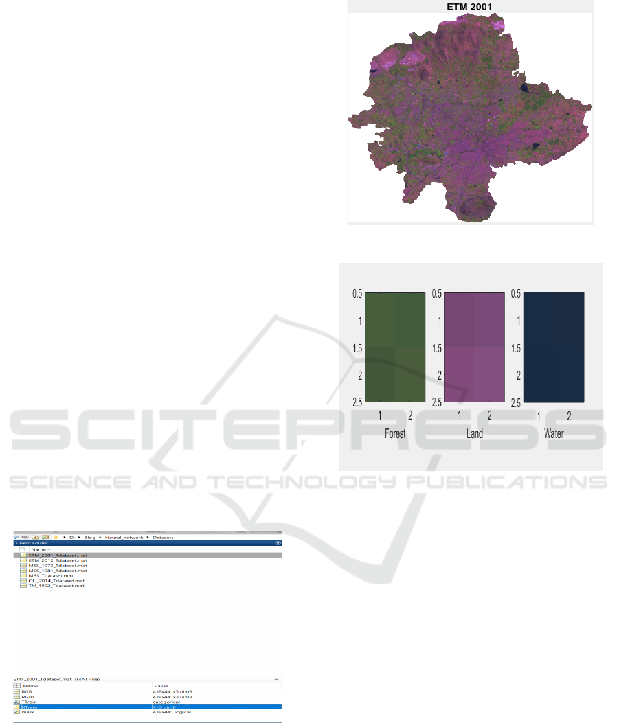
The datasets to be trained for every optical sensor

image are located in the 4-D array Figure 3. shows the

XTrain Dataset, which has pictures with dimensions

of 2x2x3xNumber_of datasets. The image has two

dimensions: height and width. The Figure 4. Shows

the RGB image has three channels. The total number

of datasets generated for every optical image is the

last component.

Figure 3: XTrain Dataset.

Figure 4: RGB Image.

Figure 5: Training Datasets for Optical Sensor Images.

The datasets generated from the optical sensor for

training are displayed in Figure 5. The class of every

2x2x3 dataset mentioned above is contained in the

categorized array known as "TTrain."

5.1.2 Training the Convolutional Neural

Network

Constructing every layer in a way that trains the

network. The initial input was the image layer. Enter

the size of the dataset, for example, 2x2x3 [2 for

height and breadth and 3 for channels since RGB].

Second place goes to the 1x1 convolution layer,

which includes three filters. The classification layer,

max pooling, SoftMax, completely connected, fully

connected, and the Rectified Linear Unit (ReLU)

function come after it.

5.1.3 Validating the Trained Datasets

In this validation stage, the accuracy of the network

that was trained will be assessed by testing 20

ICRDICCT‘25 2025 - INTERNATIONAL CONFERENCE ON RESEARCH AND DEVELOPMENT IN INFORMATION,

COMMUNICATION, AND COMPUTING TECHNOLOGIES

686

randomly selected samples against the trained

network. The 20 randomly chosen samples are

displayed in this image, together with the expected

and correct labels for each dataset. (Labels: 1 for

Forest, 2 for Land, and 3 for Water).

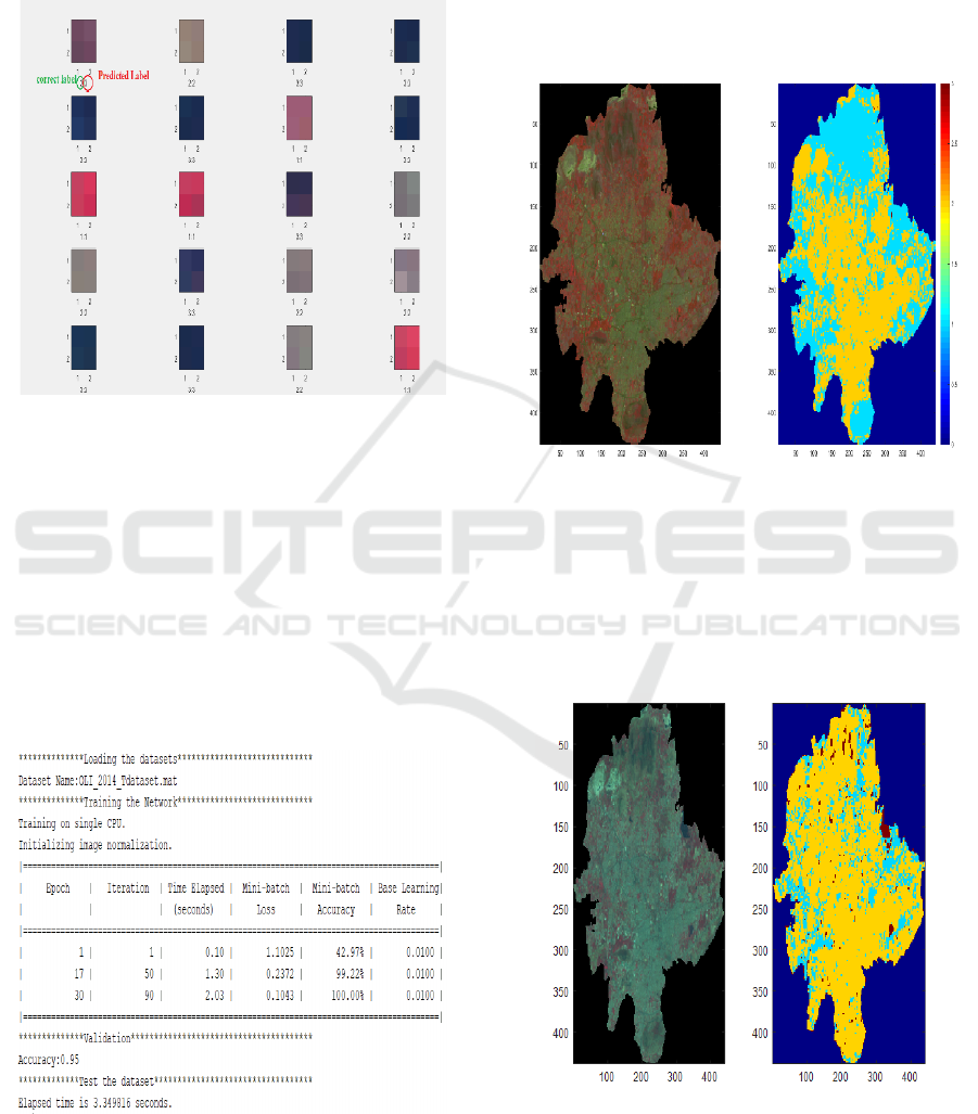
Figure 6: Confusion Matrix.

In a classification model, the confusion matrix

shows a visual comparison between the actual and

predicted labels. It has four labels (1, 2, 2.2, 3.3)

represented by four rows and columns. Every cell

displays the number of times a predicted label

(columns) was incorrect (rows). Figure 6 shows the

confusion matrix. The model's accuracy and mistakes

are measured by real positives, real negatives, false

positives, and false negatives.

5.1.4 Testing the Datasets

Figure 7: Validation Dataset.

The network that was trained will be used to test the

RGB image, and the output will be the final

categorized data. Following dataset selection,

training, and validation will occur. A calculation of

0.95% is performed for accuracy using the validation

dataset shown in Figure 7. Additionally, the accuracy

is computed after testing the twenty datasets that were

selected at random.

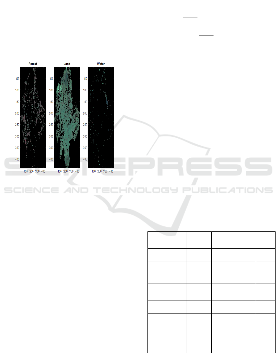
5.1.5 Final Output

Figure 8: Comparative Representation of Land Features.

The Figure 8. contrasts two images, most often

pertaining to environmental or geographic

information. The continent with colored topography

is seen in the left image. The data is visualized

utilizing a scale of colors in the right image, which

might indicate variables like height or temperature.

Figure 9: Comparative Evaluation of Vegetation Density.

Figure 9. Shows two different visual depictions of

the density of vegetation in a given area are shown in

Enhancing Optical Sensor Image Classiﬁcation through Deep Learning with Convolutional Neural Network

687

this illustration. Although the right image

represents a processed version that uses color codes

to emphasize areas of different vegetation density, the

left image looks to be an aerial or satellite view. The

map on the left displays an aerial as well as satellite

perspective, with varying green tones signifying

different vegetation types. The color-coded map on

the right most probably shows varying degrees of

density of vegetation or health, having yellow and

blue reflecting these levels. Plotting both maps on a

grid, the x and y axes have numerical scales from 50

to 400 along them.

Figure 10: Optical sensor image classification of proposed

CNN and transfer learning method.

The output images from the suggested work

demonstrate a remarkable achievement within optical

sensor image categorization, demonstrating the

model's ability to identify and classify various types

of land cover. It is shown in Figure 10. The photos are

successfully categorized into different groups like

land, water, and forest, proving the reliability of the

suggested CNN along with Transfer Learning

approach. The model's capacity to extract complex

patterns and features that occur in optical sensor

pictures is demonstrated by the clarity and accuracy

with which these classes can be distinguished. The

accurate classification's visual representation

highlights the usefulness of the suggested method and

provides insightful information for applications in

geospatial analysis, land use planning, and

environmental monitoring.

5.2 Performance Evaluation

The study employed four assessment metrics are F1-

score, accuracy, precision, and recall to analyse the

designs. These particular variables are denoted by the

numbers (11), (12), (13), and (14):

𝐴𝑐𝑐𝑢𝑟𝑎𝑐𝑦 =





(11)

𝑅𝑒𝑐𝑎𝑙𝑙 =





(12)

𝑃𝑟𝑒𝑐𝑖𝑠𝑖𝑜𝑛 =





(13)

𝐹1𝑠𝑐𝑜𝑟𝑒 =

∗∗



(14)

TP is the total amount of information that was

accurately identified as positive, regardless of the sort

of information that was positive. TN is the total

amount of data that was correctly classified as

negative even though none of the outcomes were

actually negative. The letter FN stands for the number

of variables for which the formula was wrongly

classified as negative even though the input data

showed them to be positive. False positives, or FP, are

the number of values that the algorithm misclassified

as positive even though they had been negative in the

original data. Recall is the ratio of the amount of

positive results that the algorithm determined to be

relevant to the overall amount of positive results that

were actually found during data collection. The ratio

of all the data that the model correctly classified as

positive to the total number of data that the algorithm

classified as positive is known as precision. Finally,

as previously stated, the F1-score is the harmonic

mean of recall and precision. Best of Class.

Table 1: Performance metrics of proposed CNN and

transfer learning model is evaluated with existing methods.

Method Accuracy Precision Recall

Score

Fuzzy C Means 68.9% 67% 66% 65%

Segmentation

and classification

tree method

70% 69.2% 68% 69%

Region-based

GeneSIS

89.86% 88% 87% 88%

OBIA 93.17% 93% 92% 92%

Knowledge-

ased Method

93.9% 92% 91% 93%

Proposed CNN

and Transfer

Learning

95% 94.9% 93% 94.5%

ICRDICCT‘25 2025 - INTERNATIONAL CONFERENCE ON RESEARCH AND DEVELOPMENT IN INFORMATION,

COMMUNICATION, AND COMPUTING TECHNOLOGIES

688

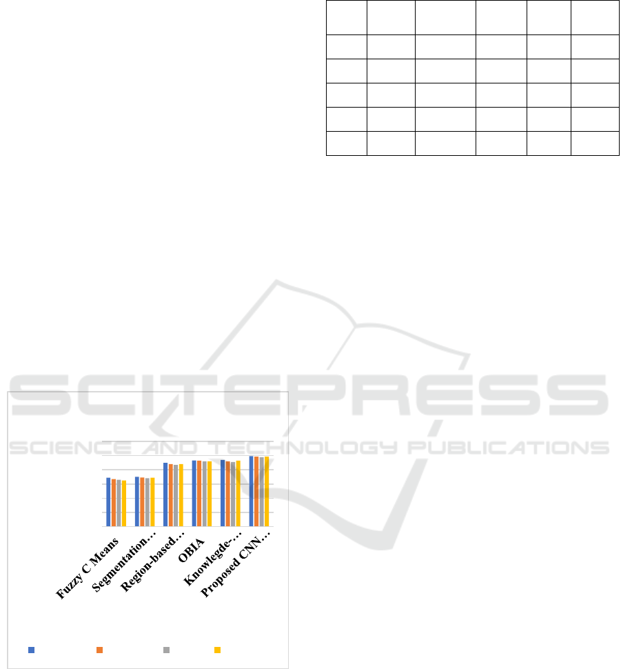
Table 1 shows a comparison of the suggested CNN

and Transfer Learning model's performance metrics

with those of the current techniques for classifying

optical sensor images. A comparative analysis of

several image classification techniques, such as the

Proposed CNN along with Transfer Learning,

Region-based GeneSIS, OBIA, Segmentation along

with Classification Tree, Fuzzy C Means, and

Knowledge-based Method, is presented in the table.

The suggested method performs better than the

others, as evidenced by the metrics accuracy,

precision, recall, as well as F1 score, which show

outstanding precision accuracy of 95%.

The findings displayed in Figure 11 demonstrate

the exceptional efficacy of the suggested model,

exhibiting a 95% accuracy rate, 94.9% precision rate,

93% recall rate, and 94.5% F1 score. By contrast,

state-of-the-art approaches like Region-based

GeneSIS & Object-Based Image Analysis (OBIA)

perform admirably, whereas conventional approaches

like Fuzzy C Means and Segmentation and

Classification Tree show reduced accuracy and

precision. Nevertheless, the knowledge-based

strategy and the suggested CNN and Transfer

Learning frameworks surpass the others, highlighting

how deep learning techniques can improve optical

sensor image categorization problems.

Figure 11: Graphical representation of proposed method

compared with existing methods.

The training log displayed offers valuable insights

into the deep learning model's training process,

including information on epochs, iterations, and time

elapsed is shown in Table 2. An epoch is a single run

over the whole training dataset, and the number of

batches

processed in an epoch is represented by its

Table 2: Proposed CNN and transfer learning model

performance.

Epoch Iteration Time

Elapsed

Mini-

atch

Mini-

atch

Base

Learning

(hh:mm:ss) Accuracy Loss Rate

1 1 1 50.00% 21.8185 0.0100

13 50 00:00:00 99.22% 0.4842 0.0100

25 100 00:00:00 99.22% 2.0046 0.0100

30 120 00:00:00 99.22% 1.0745 0.0100

iterations. Time elapsed shows how long the training

has taken overall up until a certain stage. Mini-batch

precision and loss display the results of each

iteration's effectiveness using a subset of data. The

initial learning rate used to modify model weights

through optimization is reflected in the base learning

rate. The model's development is demonstrated in the

log, with rising accuracy and falling loss, two

important measures to assess how well the training

procedure improved the classification of optical

sensor images.

5.3 Discussion

The proposed methodology is effective, as

demonstrated by the amazing 95% accuracy achieved

in Improving Optical Sensor Image categorization via

Deep Learning using Convolutional Neural

Networks. This high degree of accuracy shows how

well the model can recognize the intricate

characteristics and structures included in optical

sensor images. Using CNNs, because of their

hierarchical extraction of features capabilities, was

essential to improving the discriminative capacity of

the model. The model's ability to adapt to and perform

very well in the particular subtleties of optical sensor

image categorization was further proved by the

integration of transfer learning, which further

illustrated how good it is at utilizing prior

information. The achieved accuracy shows the

effectiveness of both the deep learning technique and

the effective fine-tuning procedure that was led by

minimizing the cross-entropy loss on the fresh

dataset. The current state of sensor image

classification systems is hindered by difficulties

managing a wide range of environmental variations

and conditions, a restricted ability to accommodate

different kinds of sensors, and a reliance on sizable

labelled datasets for efficient training (Kumarganesh.

S and M.Suganthi, 2016) and (S. K. Mylonas et al.,

2015). The ability of the suggested method to attain

0.00%

20.00%

40.00%

60.00%

80.00%

100.00%

120.00%

Methods

Performance Metrics

Accuracy Precision Recall F1 Score

Enhancing Optical Sensor Image Classiﬁcation through Deep Learning with Convolutional Neural Network

689

extraordinary accuracy demonstrates its robustness,

which is important in practical situations where

accuracy in the classification of optical sensor images

is critical. Outstanding performance is highlighted by

its flexibility, effective feature extraction using

CNNs, and knowledge leveraging. Limitations

include processing costs, dataset dependency, and

comprehension issues with its high accuracy.

Objectives include investigating data-efficient

transfer learning, improving comprehension, and

addressing computational economy. The field will

advance through standardizing evaluation measures

and dynamic adaptability to varied settings.

6 CONCLUSION AND FUTURE

SCOPE

The suggested CNN and Transfer Learning approach

shown remarkable efficacy in optical sensor image

categorization, with a remarkable 95% accuracy rate.

With the help of transfer learning to improve

classification accuracy and deep learning to facilitate

effective feature extraction, the model demonstrated

exceptional flexibility. Remarkable accuracy, recall,

and F1 score confirm its resilience in managing many

situations. Although great success was attained,

interpretability and computing resource issues were

noted. Prospective investigations ought to provide

precedence to tackling problems related to computing

efficiency by use of inventive methods, delving into

model compression without sacrificing precision.

Improving interpretability balancing explain ability

with complexity remains essential. The suggested

method's use will be expanded by looking into ways

to lessen the need for large, labelled datasets in order

to facilitate successful transfer learning. Furthermore,

the model's robustness in various optical sensor

settings should be prioritized through dynamic

adaptation to changing environmental conditions.

The field will continue to progress through

cooperative efforts to standardize evaluation

measures for optical sensor image categorization

techniques. All things considered, the suggested study

establishes a solid framework for further efforts to

maximize effectiveness, comprehensibility, and

flexibility in optical sensor image classification

systems.

REFERENCES

A. Popowicz and A. Farah, “Metastable Dark Current in

BRITE Nano-Satellite Image Sensors,” Remote Sens.,

vol. 12, no. 21, p. 3633, 2020.

A. Liu et al., “A survey on fundamental limits of integrated

sensing and communication,” IEEE Commun. Surv.

Tutor., vol. 24, no. 2, pp. 994–1034, 2022.

B, Selvalakshmi, Hemalatha K, et al. 2025. “Performance

Analysis of Image Retrieval System Using Deep

Learning Techniques.” Network: Computation in

Neural Systems, January, 1–21.

doi:10.1080/0954898X.2025.2451388.

B. Rasti and P. Ghamisi, “Remote sensing image

classification using subspace sensor fusion,” Inf.

Fusion, vol. 64, pp. 121–130, 2020.

C. Li, Y. Wang, X. Zhang, H. Gao, Y. Yang, and J. Wang,

“Deep belief network for spectral–spatial classification

of hyperspectral remote sensor data,” Sensors, vol. 19,

no. 1, p. 204, 2019.

C. Li, Y. Wang, X. Zhang, H. Gao, Y. Yang, and J. Wang,

“Deep belief network for spectral–spatial classification

of hyperspectral remote sensor data,” Sensors, vol. 19,

no. 1, p. 204, 2019.

D. Singh and B. Singh, “Investigating the impact of data

normalization on classification performance,” Appl.

Soft Comput., vol. 97, p. 105524, 2020.

D. Hong, L. Gao, J. Yao, B. Zhang, A. Plaza, and J.

Chanussot, “Graph convolutional networks for

hyperspectral image classification,” IEEE Trans.

Geosci. Remote Sens., vol. 59, no. 7, pp. 5966–5978,

2020.

F. Zhou and Y. Chai, “Near-sensor and in-sensor

computing,” Nat. Electron., vol. 3, no. 11, pp. 664–671,

2020.

Kumarganesh. S and M.Suganthi, (2016), “An Efficient

Approach for Brain Image (Tissue) Compression Based

on the Position of the Brain Tumor” International

Journal of Imaging Systems and technology, Volume

26, Issue 4, Pages 237– 242.

L. Ding, H. Tang, and L. Bruzzone, “LANet: Local

attention embedding to improve the semantic

segmentation of remote sensing images,” IEEE Trans.

Geosci. Remote Sens., vol. 59, no. 1, pp. 426–435,

2020.

L. Khelifi and M. Mignotte, “Deep learning for change

detection in remote sensing images: Comprehensive

review and meta-analysis,” Ieee Access, vol. 8, pp.

126385–126400, 2020.

M. P. Uddin, M. A. Mamun, and M. A. Hossain, “PCA-

based feature reduction for hyperspectral remote

sensing image classification,” IETE Tech. Rev., vol. 38,

no. 4, pp. 377–396, 2021.

M.-J. Huang, S.-W. Shyue, L.-H. Lee, and C.-C. Kao, “A

knowledge-based approach to urban feature

classification using aerial imagery with lidar data,”

Photogramm. Eng. Remote Sens., vol. 74, no. 12, pp.

1473–1485, 2008.

N. Thomas, C. Hendrix, and R. G. Congalton, “A

comparison of urban mapping methods using high-

ICRDICCT‘25 2025 - INTERNATIONAL CONFERENCE ON RESEARCH AND DEVELOPMENT IN INFORMATION,

COMMUNICATION, AND COMPUTING TECHNOLOGIES

690

resolution digital imagery,” Photogramm. Eng. Remote

Sens., vol. 69, no. 9, pp. 963–972, 2003.

P, Elayaraja et al. ‘An Automated Cervical Cancer

Diagnosis Using Genetic Algorithm and CANFIS

Approaches’. Technology and Health Care, vol. 32, no.

4, pp. 2193-2209, 2024.

P. Gamba and B. Houshmand, “Joint analysis of SAR,

LIDAR and aerial imagery for simultaneous extraction

of land cover, DTM and 3D shape of buildings,” Int. J.

Remote Sens., vol. 23, no. 20, pp. 4439–4450, 2002.

R. Zhang, X. Tang, S. You, K. Duan, H. Xiang, and H. Luo,

“A novel feature-level fusion framework using optical

and SAR remote sensing images for land use/land cover

(LULC) classification in cloudy mountainous area,”

Appl. Sci., vol. 10, no. 8, p. 2928, 2020.

S. K. Mylonas, D. G. Stavrakoudis, J. B. Theocharis, and P.

A. Mastorocostas, “A region-based genesis

segmentation algorithm for the classification of

remotely sensed images,” Remote Sens., vol. 7, no. 3,

pp. 2474–2508, 2015.

S. Bera and V. K. Shrivastava, “Analysis of various

optimizers on deep convolutional neural network model

in the application of hyperspectral remote sensing

image classification,” Int. J. Remote Sens., vol. 41, no.

7, pp. 2664–2683, 2020.

X. Lei, H. Pan, and X. Huang, “A dilated CNN model for

image classification,” IEEE Access, vol. 7, pp. 124087–

124095, 2019.

Y. Xu et al., “Advanced multi-sensor optical remote

sensing for urban land use and land cover classification:

Outcome of the 2018 IEEE GRSS data fusion contest,”

IEEE J. Sel. Top. Appl. Earth Obs. Remote Sens., vol.

12, no. 6, pp. 1709–1724, 2019.

Y. Feng, Z. Chen, D. Wang, J. Chen, and Z. Feng,

“DeepWelding: A deep learning enhanced approach to

GTAW using multisource sensing images,” IEEE

Trans. Ind. Inform., vol. 16, no. 1, pp. 465–474, 2019.

Y. Bazi, L. Bashmal, M. M. A. Rahhal, R. A. Dayil, and N.

A. Ajlan, “Vision transformers for remote sensing

image classification,” Remote Sens., vol. 13, no. 3, p.

516, 2021.

Y. Sun, B. Liu, X. Yu, A. Yu, K. Gao, and L. Ding,

“Perceiving spectral variation: Unsupervised spectrum

motion feature learning for hyperspectral image

classification,” IEEE Trans. Geosci. Remote Sens., vol.

60, pp. 1–17, 2022.

Z. Zhao, J. Li, Z. Luo, J. Li, and C. Chen, “Remote sensing

image scene classification based on an enhanced

attention module,” IEEE Geosci. Remote Sens. Lett.,

vol. 18, no. 11, pp. 1926–1930, 2020.

Enhancing Optical Sensor Image Classiﬁcation through Deep Learning with Convolutional Neural Network

691