Predictive Quality of In-Fabrication Products in Smart Manufacturing

Using Graph-Based Deep Learning

Peter Davison

1,2 a

, Muhammad Fahim

1 b

, Roger Woods

2 c

, Scott Fischaber

, Marcus Haron

and Cormac McAteer

Centre for Intelligent Sustainable Computing, Schools of Electronics, Electrical Engineering and Computer Science,

Queen’s University Belfast, Belfast, Northern Ireland, U.K.

Analytics Engines Ltd., 1 Chlorine Gardens, Belfast, Northern Ireland, U.K.

Seagate Technology, 1 Disk Drive, Derry/Londonderry, Northern Ireland, U.K.

ﬁ

Keywords:

Graph Neural Network, Semiconductor Wafers, Heterogeneous Graphs, Knowledge Graphs, Graph Readout,

Graph Classiﬁcation.

Abstract:

Graph neural networks are a very powerful way to learn about relationships between entities in graphs.

With the rise of IoT devices in manufacturing, more data is being collected to minimise the waste of both

valuable resources and time for fabrication. In this paper, we introduce a methodology for predictive quality

of in-fabrication products using graph neural networks. Data is collected from a live-working semiconductor

wafer fabrication facility and used to produce heterogeneous graphs that represent the fabrication timeline

of a wafer. The model uses the graph attention network architecture to classify whether a timeline is scrap

or non-scrap. It uses historical graph-level labelled data and achieves an F1-score of 0.928, compared to

baselines models of a LSTM and a Homogeneous Graph Attention Network with scores of 0.424 and 0.786

respectively. It gives a foundational framework for future anomaly detection with semiconductor fabrication,

allowing real-world data to be analysed with graph-based deep learning tools to provide interpretation and

accessible graph-based results.

1 INTRODUCTION

The rise of both the Internet of Things (IoT) and

Artiﬁcial Intelligence (AI) has had an impact in

many different sectors. As more industries are

evolving into the “Fourth Industrial Revolution” or

“Industry 4.0”, they are capitalising on a multitude

of multivariate sensors monitoring aspects in their

environment, resulting in large volumes of data,

which contain anomalies. Smart factories house

extensive fabrication lines, harnessing the power of

Industrial Internet of Things (IIoT), but, like many

other industries, still face the challenge of detecting

anomalies, which is the focus of this work.

Approaches to solve the Anomaly Detection

(AD) problem in IoT have revolved around

combining different Artiﬁcial Neural Network

https://orcid.org/0009-0007-4648-9015

https://orcid.org/0000-0001-6259-5458

https://orcid.org/0000-0001-6201-4270

(ANN) architectures (Wu et al., 2022). These

have issues, however, when focusing speciﬁcally

on high-dimensional datasets, often present in

Multivariate IoT data. They cannot scale efﬁciently,

and thus capture the temporal dependencies that are

imperative for real-world cases.

In our research, real-world private data

from Seagate Technology’s fabrication facility

in Springtown is utilised. Homogeneous and

heterogeneous graphs have been created, resulting in

a total of 1652 graphs representing the fabrication

process from start to ﬁnish or a scrap event. This

work proposes a Graph Neural Network (GNN)-based

model to identify whether a fabrication timeline of

data of an in-fabrication product contains anomalous

metrology readings. The main aim is to explore

the use of graph-form data structures for analysis

and measure the efﬁcacy of anomaly detection in

semiconductor wafer fabrication.

The manufacturing (Atherton and Atherton, 1995)

process comprises 1000s of steps, with some

Davison, P., Fahim, M., Woods, R., Fischaber, S., Haron, M. and McAteer, C.

Predictive Quality of In-Fabrication Products in Smart Manufacturing Using Graph-Based Deep Learning.

DOI: 10.5220/0013855100003982

Paper published under CC license (CC BY-NC-ND 4.0)

In Proceedings of the 22nd International Conference on Informatics in Control, Automation and Robotics (ICINCO 2025) - Volume 1, pages 145-153

ISBN: 978-989-758-770-2; ISSN: 2184-2809

145

processes needing to work at micrometre precision;

therefore, extensive metrology is applied to ensure

quality. In this work, measurements from each sensor

in the metrology process tools are transformed into

a heterogeneous graph. In this graph, each process

tool creates a local neighbourhood of its sensors with

nodes and edges, and a transferral between tools is

shown by a directed edge from one process tool node

to the next (Fig. 1). The graphs have a total upwards

of 300 unique process tools that are possible in any

order, resulting in about 6500 distinct edge types in

the heterogeneous graphs.

The work makes the following contributions:

1. Using graph-based format, our GNN model can

analyse intricate characteristics in sensor data,

by identifying inconsistencies that may produce

a graph-level scrap event for the semiconductor

wafer in-fabrication.

2. The experiments are performed on real-dataset,

and the proposed GNN model achieves an

F1-score of 0.928, which, to our knowledge,

outperforms other state-of-the-art graph-based

methods used for graph-level classiﬁcation in

semiconductor wafer fabrication.

3. This work provides a foundational model

for semiconductor wafer fabrication, with

interpretable and accessible graph-based results

for further study.

The rest of this paper is organised as follows:

Section 2 provides background on GNNs and current

methodologies used in AD in smart manufacturing;

Section 3 outlines the methodology and gives

information on the dataset, the model architecture

and the training process; Section 4 details the

experimental setup and results and; Section 5

concludes the paper and discusses potential future

work.

2 BACKGROUND

2.1 Graph Neural Networks

Artiﬁcial neural networks have the ability to represent

and classify structured data. Scarselli et al. (Scarselli

et al., 2009) extended the concept by introducing

GNNs, along with methods to encode acyclic, cyclic,

directed and undirected graphs. GNNs can learn the

relationships between variables (inter-variable) and

the relationship between datapoints (intra-variable).

This is crucial in many real-world applications where

variables are not isolated but can be inﬂuenced

by each other; this is leveraged in GNNs by

understanding the interactions between the variables.

Additionally, intra-variable relationships can reveal

patterns in a variable’s data over time which is

imperative in the analysis.

GNNs graphs are either homogeneous or

heterogeneous. Homogeneous graphs (Homographs)

contain only one type of node and edge taking the

same number of features for all nodes, but, in turn,

apply the same meaning for every feature of the nodes

and edges. Heterogeneous graphs (Heterographs)

contain multiple node and edge types, therefore

containing more information, either new relevant

pieces of a pattern, or additional layers of complexity

and noise which can increase the difﬁculty and

time needed to train the model (Labonne, 2023).

Heterogeneous graphs, however, can represent

real world aspects more effectively, such as in

manufacturing where different machines can contain

different sensors that could be more signiﬁcant when

it comes to identifying patterns.

The process of creating accurately representative

graphs is data driven, whereby core features include

events and locations as nodes, and the relationships

and interactions between them are represented as

edges. Due to the dependency on the data, creating

an effective graph can be difﬁcult, requiring domain

expertise to ensure the data is correctly represented.

A poorly created graph can lead to a poorly trained

model, as the model may misinterpret the content.

Depending on the graph and it’s usage, it may

be referred to as Information Networks, Interaction

Networks, Knowledge Graphs (KGs), but we will

simply call them graphs.

Graph classiﬁcation, or graph-level readout, is

a classiﬁcation level involved in GNNs, the others

being node and edge classiﬁcation. It classiﬁes a

graph using a GNN model that contains pooling

methods which aggregate graph embeddings to give a

result. It can be efﬁciently used in various disciplines.

In (Wen et al., 2024), GNN-based methods are used

to track machine wear-and-tear, giving an accurate

tracking system to indicate when machines need

maintenance.

2.2 Smart Manufacturing Anomaly

Detection

Anomaly detection in manufacturing is indispensable,

with the potential for deviations of an assembly line

increasing with the complexity of products; the more

steps in a process suggests that more problems may

occur. Anomalies still arise in some of the most

advanced facilities in the world, so efﬁcient AD is

essential. Proactive AD can maintain high levels

ICINCO 2025 - 22nd International Conference on Informatics in Control, Automation and Robotics

146

of quality and operational efﬁciency, ensuring that

manufacturing companies can meet market standards

as well as shortages.

Current AD methodologies using techniques

that are not graph-based in IIoT include extensive,

spanning Long Short-term Memory (LSTMs),

Auto-Encoders (AEs), Convolutional Neural

Networks (CNNs), and hybrids. An AE-based

Digital Twin model (Jeon et al., 2024) is used

for “Extreme Rare Anomalies” in the fabrication

process, yielding a high F1-score of 0.955. An

LSTM-based Autoencoder (Hwang et al., 2023)

works on anonymised wafer fabrication data from

the industry, whereas (Hsieh et al., 2019) uses an

LSTM-based Autoencoder with an extensive outline

of the current problems with wafer fabrication

anomaly detection, to achieve an F1-score of 0.924.

Although the aforementioned methodologies are

efﬁcacious in their use case, they do not suite the

aims of this literature with regards to achieving

graph-based deep learning anomaly detection.

GNNs have also been applied for AD smart

manufacturing, where (Wu et al., 2022) has presented

examples from different sectors in IIoT, including

a Smart Factory, with basic models. Whilst being

deployed in great use cases, the models are more

of a proof of concept. Guan et al. (Guan

et al., 2022) implements a Temporal Convolutional

Network (Bai et al., 2018) and the Graph Attention

Network GATv2 (Brody et al., 2022) effectively

detects anomalies in the Mars Science Laboratory,

Soil Moisture Active Passive, and the Server Machine

datasets with F1-scores upwards of 0.95. Although

the proposed is a good architecture, Guan et al.

mostly outlines example use cases and semi-relevant

public datasets. Cassoli et al. (Cassoli et al., 2023)

uses Knowledge Graph creation (Bretones Cassoli

et al., 2022) to effectively implement a graph creation

pipeline for raw metrology manufacturing data and

feed this into a GNN achieving scores of 0.48. To our

knowledge, this work is the closest to this literature as

it uses metrology data from a smart factory to create

knowledge graphs and a GNN to detect graph-level

anomalies.

Cassoli et al. create Knowledge Graphs from

the public Bosch dataset

in a similar way to that

in Section 3.2, to create a timeline of events

with manufacturing data. Although the methods

are similar, (Cassoli et al., 2023) achieves an

F1-score of 0.48, suggesting that the GraphSAGE

architecture may not be as suitable for the task of

Bosch Production Line Performance

https://www.kaggle.com/competitions/

bosch-production-line-performance

graph classiﬁcation versus the later explored Graph

Attention Network model.

As shown, there has been extensive work

surrounding AD in smart manufacturing, using both

non-graph and graph-based methods. However, we

believe there is a gap in current research surrounding

a foundational model that can identify anomalies in a

timeline of graph-based metrology data. This would

supply an opportunity for interpretable and accessible

GNN results, with inherent access to graph-based

visualisations through the nature of the graph-form.

Using a real-world use case from industry partners

Seagate Technology, we demonstrate the application

for this type of model on real-world data.

3 METHODOLOGY

3.1 Fabrication Dataset

The data is taken from one of two of Seagate’s

semiconductor wafer fabrication facilities in

Springtown, which manufactures read/write heads

for hard disk drives. It contains over 1000 steps and

can frequently reach over 70 unique machines

, with

many more Quality Control (QC) checks involving

engineer-set thresholds. These QC checks use

data from inspection stations, or process tools, that

contain many different types of metrology sensors

to execute miniscule measurements on the wafers

in the area of one nanometre. Certain sensors can

be the same type yet may have different parameters,

measuring important features on the wafer such

as thickness, uniformity and topology. However,

like any smart factory, the fabrication process can

suffer from defects through many different sources.

These defects can be caused by the equipment, the

environment, the materials, or the process itself.

The data from the QC checks are not always

indicative of the source of the defect and can be

challenging to interpret. When a defect occurs, the

wafer is pulled and inspected by an engineer to

determine if the wafer is nominal, can be reworked,

or if it must be scrapped. The latter two options

then involve a data science team to investigate the

root cause of the defect, which can be a very

time-consuming process and potentially costly to

any more faulty wafers produced. An example of

a fault that occurred in the past involved a dry

etching machine that was not functioning correctly

Springtown – A Hard Drive Factory Like

No Other https://www.silicon.co.uk/workspace/

springtown-a-hard-drive-factory-like-no-other-119580

Predictive Quality of In-Fabrication Products in Smart Manufacturing Using Graph-Based Deep Learning

147

and became obstructed with etched debris. This

led to the machine to cause defects in the wafers

it processed, which was a root cause that was not

immediately obvious from the QC data.

The data is a collection of fabrication processes

of wafers from the metrology sensors on the line,

either from start to ﬁnish or up to when the wafer

was scrapped. For example, if a wafer completes

fabrication without a serious error then the metrology

timeline data will be from the ﬁrst process to the

very end when the wafer completes fabrication in the

facility. On the other hand, if a wafer is ﬂagged for

a fault or an error occurs with a machine and the

wafer is pulled out of the fabrication by a technician,

the data shall be from the ﬁrst process to the last

process that ﬂagged the wafer, or an adjacent process

that occur at the same time, and stopped fabrication.

Working with the partners at Seagate Technology,

this literature aims to aid in the investigation and

explanation of anomalies in the metrology data by

creating a foundational framework through the means

of a graph-based model that can identify graph-level

anomalies in the metrology timeline of fabrication

data.

3.2 Graph Creation

Due to the nature of metrology data being raw data,

preprocessing is necessary. The wafer fabrication

data is formatted ﬁrst into a PostgreSQL database

which supports efﬁcient future data appendage for

new data and querying for data retrieval, with each

fabrication timeline being assigned a unique ID. This

is the ﬁrst foundation of the framework, allowing

the graphs for the GNN to be created. The data is

then queried and formatted into graph-structured data

using Python and the Pytorch Geometric library

A homograph G = (V , E) is composed of its

set of nodes (or vertices) V = {1,..., N} and edges

E, where (i, j) ∈ E denotes a directed edge from

node, i, to node, j. Each node i ∈ V contains an

initial node representation h

∈ R

, where d is the

size of the feature matrix. Due to the heterogeneity of

real-world data, however, a heterograph is more ﬁtted

for an accurate representation of the metrology data.

It allows the set of nodes V to contain different types

of nodes, such as sensors or machines, that contain

different dimensions for the feature matrix, and

allows for the possibility to have different coefﬁcients

for each type.

A directed heterograph is deﬁned as G = (V , E),

where each node i ∈ V and each edge (i, j) ∈ E are

Pytorch Geometric https://pytorch-geometric.

readthedocs.io/en/latest/index.html

associated with mapping functions φ : V → T and

ψ : E → R respectively, with both nodes and edges

requiring a type: φ(v) ∈ T and ψ(e) ∈ R respectively

(Sun and Han, 2013). T and R denote the set of

node and edge types, where |T | + |R| > 2 to result

in a heterogeneous graph. Each node still contains

an initial node representation, but with the addition

of a node type h

(t)

∈ R

, where d

is the number

of features for node type t. In the graph, each edge

type is formed by both endpoint node and relationship

types.

There are three relationship types:

HAS PROCESS, PROCESS OF and TRANSFER.

The two former types are used to represent the edge

between a process tool, or machine, node and a data

node, whereas the latter is used to represent the edge

between two process tool nodes, shown in Fig. 1.

Although heterogeneous graphs are a more accurate

representation of the metrology data, they contain

a complex structure that can cause problems for

execution times and model complexity. This issue is

discussed further in Section 3.3.

mach2mach1

TRANSFER

HAS_PROCESS

PROCESS_OF

...

Figure 1: An example directed heterogeneous graph snippet

containing machine 1 and machine 2 nodes with a process

data node of machine 1.

As previously mentioned, the technical

implementation of the graph creation involves

the use of the Pytorch Geometric library to create

the graphs. Scripts pull data from the PostgreSQL

database for each wafer fabrication timeline ID,

ordering the metrology data by process timestamp.

Python scripts then format this into the directed

heterograph, creating a sub-graph for each process

tool in the fabrication process with child nodes as

data nodes containing the metrology readings from

sensors. The metrology readings are normalised

using Min-Max scalers when added to ensure there

are no scaling issues or biased results resulting from

the varying value ranges from each node type. Each

sub-graph has a central parent node to represent the

process tool, as an endpoint of a directed edge from

the previous process tool and continuing the ﬂow

with a directed edge to the following process tool

node in the fabrication process; this represents the

transferral of the wafer through each machine on the

fabrication line. An example of the overall process

for one timeline is abstracted in Fig. 2.

ICINCO 2025 - 22nd International Conference on Informatics in Control, Automation and Robotics

148

Timeline_id

pdatetime

Machine_id

Stage_id

Step_id

...

meas_avg

targ_avg

4c8672d6-

af1a-4dce

2024-08-15

17:40:28

mach1

stage1

step1

...

0.9359

4c8672d6-

af1a-4dce

2024-08-15

17:40:28

mach1

stage1

step2

...

0.7708

...

4c8672d6-

af1a-4dce

2025-02-03

06:56:27

mach95

stage25

step150

...

245.427

250

4c8672d6-

af1a-4dce

2025-02-03

06:56:27

mach95

stage25

step150

...

248.836

250

...

mach95

mach1

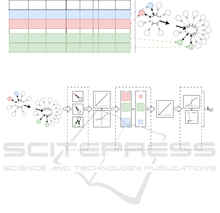
Figure 2: Example of a wafer fabrication timeline being converted into a directed heterogeneous graph, showing the ﬁrst and

last process tool sub-graphs. Example colours are used to show different types of sensors, with an example of the same sensor

type (green) executing two metrology measurements. Please note, there are many features that result from the metrology

readings and are added as node features in the graphs, but for conﬁdentiality reasons we have only added a selection of

high-level features as an example.

...

mach95

mach1

Edge-type-specific

GAT convolutional

operator list

Linear Transformation

& Activation Function

Node-type-specific

mean pooling and

significance weight

application layer

...

Input Data

...

Linear Transformation

into single scalar value

graph representation

Sigmoid function

into threshold

binary classification

Figure 3: The pipeline of the graph-level classiﬁcation model, HeteroGAT, with the three main layers outlined.

3.3 Graph Neural Network

Architecture

To classify anomalies that occur in the metrology

data, a GNN graph-level classiﬁcation model is used,

herein referred to as HeteroGAT. This allows the user

to easily identify which fabrication timelines contain

anomalous metrology data that need investigation.

To achieve this, HeteroGAT contains three main

layers: 1) the Graph Attention Network (GATv2)

(Brody et al., 2022) Convolutional operator list, 2) the

Pooling layer, and 3) the Graph Classiﬁcation layer.

Fig. 3 shows the overall pipeline, with the three

main layers outlined with dashed rectangles. The

GNN architecture was chosen as it was estimated that

HeteroGAT could provide unique insights into the

fabrication process, such as potential cross-machine

relationships that would aid in the analysis of defects.

The ability of GNNs to set a foundation for its results

to be explained in an interpretable way through the

use of the graph-based data was also a key factor in

architecture choice.

GAT Convolutional Operator List. This layer

contains a list of GATv2Conv operators with

an individual operator for each edge type in

the heterogeneous graphs, therefore following the

construction deﬁned in (Brody et al., 2022) with

some alterations to incorporate the heterogeneity of

the graphs. Each edge type requires an individual

operator which captures the unique information that

the edges possess with a learnable weight matrix

, thus dramatically increasing the complexity

compared to homogeneous models. For any given

node, i, there is a relation-speciﬁc neighbourhood,

(r)

, of relation, r, that contains the set of nodes

(r)

= { j ∈ V |(i, j) ∈ E ∧ ψ(i, j) = r}. Each

type-speciﬁc neighbourhood of type r is passed into

a scoring function that computes the importance of

the neighbour features in j to the node i:

(r)

i j

= a

⊤

(r)

LeakyReLU



(r)

∥W

(r)



(1)

where a

⊤

(r)

is a learnable relation-speciﬁc attention

vector, h

and h

are the previously mentioned

node representations and ∥ denotes the concatenation

operation.

The attention scores from equation (1) are then

normalised across all neighbours of node i with a

Predictive Quality of In-Fabrication Products in Smart Manufacturing Using Graph-Based Deep Learning

149

softmax function:

(r)

i j

exp



(r)

i j



∑

′

∈N

(r)

exp



(r)

i j

′



(2)

Then, the node representation, h

, is updated by

aggregating the neighbourhood information over all

relations with the attention coefﬁcients:

= σ







∑

r∈R

∑

j∈N

(r)

i j

(r)







(3)

where σ is the non-linearity. Contrary to other

popular models, multi-head attention mechanism is

not used. While, this mechanism would be useful

in homogeneous models that focus on the same

data, HeteroGAT already breaks down the graphs

into their type-speciﬁc neighbourhoods; this has the

same impact as achieving a multi-head attention

mechanism. Addition of such a mechanism could

extend the ability of each type-speciﬁc operator, but it

would increase the complexity and potentially involve

overﬁtting.

Pooling and Signiﬁcance Weight Application

Layer. The graph pooling, or graph-level readout,

classiﬁes the graph and thus allows for further

investigation if the classiﬁcation for the graph is

anomalous. In this speciﬁc use case, the label denotes

the fabrication timeline’s prediction; 1 means it is

marked for scrap and 0 as nominal. A mean is taken

across all node representations for each node type,

then concatenated to form a list of type-speciﬁc mean

node representations. This list is then multiplied

against type-speciﬁc learnable weights, S

, that denote

the signiﬁcance of the node type with regards to the

graph-level classiﬁcation and passed into the ﬁnal

Linear Transformation that give a scalar value for

classiﬁcation. In training, h

is compared to the

graph-level y-value, that is provided by the industry

partners to deem the fabrication timeline’s destiny,

to calculate the loss using a Binary Cross-Entropy

(BCE) loss function.

Graph Classiﬁcation Layer. This ﬁnal layer uses a

threshold set by the user to classify if the graph-level

readout from the pooling layer shows an anomalous

label of 1 or a nominal label of 0.

4 EXPERIMENTS & RESULTS

4.1 Experimental Setup

The hardware setup used for this literature included

the CPU Xeon E3-1200 v3 3.10GHz Processor with

32GB RAM and the GPU Nvidia GeForce RTX 2080

Ti 11GB.

The graph datasets contain 1652 graphs, of which

1393 are non-scrap timelines labelled 0, and 259 are

scrap timelines labelled 1.The dataset is split into a

training, validation and testing set with a ratio of

60:20:20.

For comparison, a basic LSTM model and a

basic Homogeneous Graph Attention Network

(HomoGAT) are used with some optimal

hyperparameter searching. The LSTM uses the

raw, non-graph data, as a more traditional machine

learning technique for similar sequence data would

use; a single LSTM operator results in a value for the

“sequence” representation. The HomoGAT, similarly

to HeteroGAT, contains a GATv2Conv operator and

is followed by the graph readout function. For the

data to be processed by HomoGAT, there cannot be

multiple node types; therefore, a homogeneous graph

dataset of the same fabrication data is used. As seen

in Fig. 4, the sub-graphs representing the machines

are complete (Labonne, 2023), as opposed to in the

heterogeneous dataset where each sub-graph having

a machine-typed node in the centre. There is also an

edge between every node representing the order using

process timestamps, as seen between each sub-graph.

All models are then followed by a sigmoid function

and a threshold to result in a binary classiﬁcation for

their respective data form, either graph or sequence.

As mentioned, the loss function being used is the

BCE loss. As usual with a real-life dataset for binary

classiﬁcation, there is a very large class imbalance

towards non-scrap timelines, therefore the positive

weight for the BCE loss function is set to 259/1393 =

0.1859. The optimiser used is the Adaptive Moment

Estimation (ADAM) optimiser. The learning rate

is also reduced on a plateau with a patience of 10.

The batch size is set to 1 as the task is graph-level

classiﬁcation. All hyperparameters are seen in Table

4.2 Results

As shown in Table 2, all models performed well with

the highly advanced Seagate data, with HeteroGAT

resulting in the highest F1-score of 0.928. The

power of the HeteroGAT is the foundation it sets with

potential in a model that is more interpretable, as

explored hereinbelow. However, HeteroGAT suffers

with extremely long training times compared to the

baseline models, with the experimental setup running

for ∼ 20 hours with our hardware, compared to ∼ 0.5

hours for HomoGAT and ∼ 5.5 hours for the LSTM.

Although the training phase is commonly a single

ICINCO 2025 - 22nd International Conference on Informatics in Control, Automation and Robotics

150

Flow of fabrication timeline graph

Metrology data nodes

Process tool complete subgraph

Order-representing

directed edge

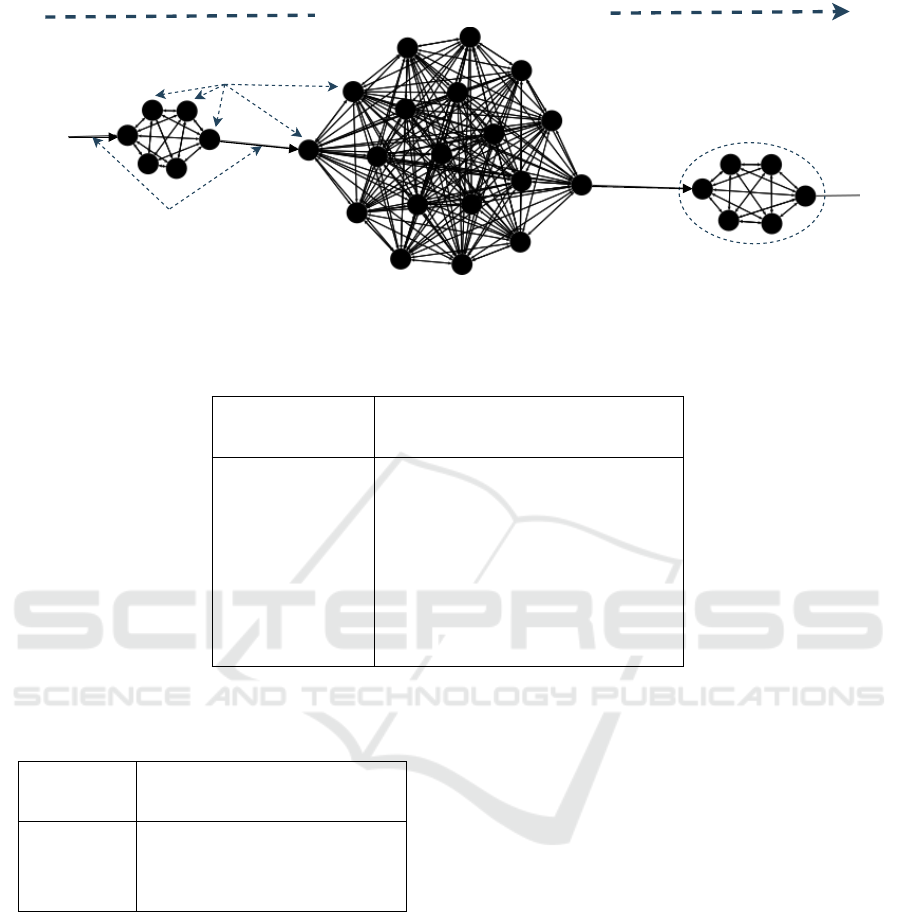
Figure 4: Annotated extract of a wafer fabrication timeline in the directed homogeneous graph-form used in the HomoGAT. It

contains three process tool sub-graphs and one node type denoted with one colour (black) showing the lack of representation

for sensor types compared to the heterogeneous graph in Fig 1.

Table 1: Model hyperparameters for heterogenous GAT, homogeneous GAT, and LSTM model.

Hyperparameter Value

HeteroGAT HomoGAT LSTM

Batch Size 1 1 1

Hidden Channels 64 96 16

Dropout 0.5 0.5 0.5

Learning Rate 10

−3

Positive Weight 0.1859 0.1859 0.1859

Threshold 0.4 0.5 0.5

Epochs 30 30 30

Table 2: Model performance metrics for our proposed

HeteroGAT and comparison with baseline models on the

Seagate dataset.

Model Metrics

Precision Recall F1-Score

HeteroGAT 0.970 0.889 0.928

HomoGAT 0.708 0.885 0.786

LSTM 1.000 0.269 0.424

occurrence, if machines are added to the fabrication

process, training would potentially need to be rerun

or a system that could integrate new operators to the

model efﬁciently would be needed.

HeteroGAT is able to classify the timelines with a

high level of accuracy, and if applied to a live system

would be able to identify in-fabrication products that

contain anomalous data and need inspection. This

would be executed by feeding the model a graph

of the fabrication metrology timeline data whilst the

product is still on the fabrication line, and if the model

classiﬁes a scrap timeline, the coinciding product

could be removed from the line and inspected.

4.3 Time Complexity

A large issue with the current architecture of

HeteroGAT is the model’s time complexity. Each

edge type requires its own GATv2 operator, therefore

requiring its own learnable parameters so the model

scales with the number of edge types in all of the

graphs present in the graph dataset. Let V be the set

of nodes, E be the set of edges, R be the set of edge

types, d be the node feature matrix dimensions, d

′

the hidden channels dimension in GATv2 which we

shall assume to be constant for all GATv2 operators.

We shall be using the stated complexity of GATv2

from their paper (Brody et al., 2022):

O(|V |dd

′

+ |E|d

′

) (4)

For every edge type in R , there is a GATv2 operator,

therefore let the set of node types involved in the

edge type r be S

. Included is also the differing node

type feature dimensions for node types T . We are

also assuming the number of GATv2 layers L = 1,

therefore:

∑

r=1

∑

t∈S

· d

′

(5)

Predictive Quality of In-Fabrication Products in Smart Manufacturing Using Graph-Based Deep Learning

151

Then, including the dominant cost of the node type

linear transformation, results in the ﬁnal dominant

time complexity of HeteroGAT:

∑

r=1

∑

t∈S

′

∑

t=1

′2

(6)

The other modules of the model are not as dominant

as the linear transformation therefore have not been

included. Equation 6 shows the models complexity is

heavily dominated by the number of edge types in the

graph dataset, and therefore suggest that techniques

such as basis-decomposition (Schlichtkrull et al.,

2017) would beneﬁt here to improve efﬁciency.

5 CONCLUSION AND FUTURE

WORK

In this paper, we introduced a framework to create

Heterogeneous Graphs from separated metrology

data sources on a fabrication line and apply a

GNN-based model to classify an on-line product

as either nominal or anomalous, suggesting a scrap

action. By utilising past scrap and non-scrap timeline

data, our model can learn the relationships between

the different machines and sensors, as well as the

signiﬁcance of those types on the overall product

quality. We show that our model can classify

the product with high accuracy; however, more

importantly, we contribute a new foundation for

future work in exploring graph-based deep learning

with a rapidly advancing ﬁeld like semiconductor

fabrication. The ability to utilise metrology data

from a fabrication facility with graph-based deep

learning opens up many possibilities for improved

anomaly detection and management within active

manufacturing, with high model performance as well

as knowledge graph capabilities. This framework’s

nature of being graph-based allows for efﬁcient

creation of the visualisations of input and output data

that would be highly effective for a digital twin-like

tool for operators to use in their decision-making

processes, allowing for a pathway to efﬁcient

explainable AI. In addition to showing that this

method is effective in identifying issues, we provide a

valuable service to the real-world industrial partners

at Seagate Technology by aiding their anomaly

detection processes.

5.1 Future Work

To further build on the work completed in

this literature, future work shall include node

classiﬁcation for an in-depth root cause analysis

of the anomalies, allowing for a hyperspeciﬁed

location of the issue. Moreover, we shall explore

other GNN architectures, such as GraphSAGE,

Graph Deviation Networks and Relational Graph

Convolutional Networks, as well as the alteration

of the graph creation process to explore whether

including additional information to aspects such

as edges or metapaths can improve the model’s

performance. On top of this, a formal deﬁnition

of the temporal aspect of the data must be added,

whether that be through the graphs structure using

possibilities like PyTorch Geometric’s TemporalData

class, or using architectures such as the Temporal

Heterogeneous GNN (Wen et al., 2024). The models

training times are a big issue, therefore a new graph

pipeline using the Deep Graph Library (DGL) (Wang

et al., 2020) shall be implemented and running times

will be compared with the current PyTorch Geometric

library implementation.

5.2 Ethical Concerns

We would like to highlight that the framework

introduced could be used to supplant jobs, however,

this is not the intention of this work. The goal of this

research is to provide a tool to assist human operators

in their decision-making and investigation processes

of increasingly complex systems.

ACKNOWLEDGEMENTS

We would like to thank UKRI for support through the

SmartNanoNI Strength in Places Funded project and

the EPSRC Doctoral Training Partnership.

REFERENCES

Atherton, L. F. and Atherton, R. W. (1995, November

30). Wafer Fabrication: Factory Performance and

Analysis. Springer Science & Business Media.

Bai, S., Kolter, J. Z., and Koltun, V. (2018, April 19).

An Empirical Evaluation of Generic Convolutional

and Recurrent Networks for Sequence Modeling.

arXiv: 1803.01271 [cs]. https://doi.org/10.48550/

arXiv.1803.01271

Bretones Cassoli, B., Jourdan, N., and Metternich, J.

(2022) Knowledge Graphs for Data And Knowledge

Management in Cyber-Physical Production Systems.

https://repo.uni-hannover.de/handle/123456789/

12278

Brody, S., Alon, U., and Yahav, E. (2022, January

31). How Attentive are Graph Attention Networks?

ICINCO 2025 - 22nd International Conference on Informatics in Control, Automation and Robotics

152

arXiv: 2105.14491 [cs]. https://doi.org/10.48550/

arXiv.2105.14491

Cassoli, B. B., Jourdan, N., and Metternich, J. (2023)

Multi-source data modelling and graph neural

networks for predictive quality. 120:39–44. https:

//doi.org/10.1016/j.procir.2023.08.008

Guan, S., Zhao, B., Dong, Z., Gao, M., and He, Z.

(2022) GTAD: Graph and Temporal Neural Network

for Multivariate Time Series Anomaly Detection.

24(6):759. https://doi.org/10.3390/e24060759

Hsieh, R.-J., Chou, J., and Ho, C.-H. (2019) Unsupervised

Online Anomaly Detection on Multivariate Sensing

Time Series Data for Smart Manufacturing. In

2019 IEEE 12th Conference on Service-Oriented

Computing and Applications (SOCA), pages 90–97.

https://doi.org/10.1109/SOCA.2019.00021

Hwang, R., Park, S., Bin, Y., and Hwang, H. J.

(2023) Anomaly Detection in Time Series

Data and its Application to Semiconductor

Manufacturing. 11:130483–130490. https:

//doi.org/10.1109/ACCESS.2023.3333247

Jeon, M., Choi, I.-H., Seo, S.-W., and Kim, S.-W.

Extremely Rare Anomaly Detection Pipeline in

Semiconductor Bonding Process With Digital

Twin-Driven Data Augmentation Method.

14(10):1891–1902. https://doi.org/10.1109/TCPMT.

2024.3454991

Labonne, M. Hands-On Graph Neural Networks Using

Python: Practical Techniques and Architectures for

Building Powerful Graph and Deep Learning Apps

with PyTorch. Packt Publishing Ltd.

Scarselli, F., Gori, M., Tsoi, A. C., Hagenbuchner, M.,

and Monfardini, G. The Graph Neural Network

Model. 20(1):61–80. https://doi.org/10.1109/TNN.

2008.2005605

Schlichtkrull, M., Kipf, T. N., Bloem, P., family=Berg,

given=Rianne, p. d. u., Titov, I., and Welling, M.

Modeling Relational Data with Graph Convolutional

Networks. arXiv: 1703.06103 [cs, stat]. https://doi.

org/10.48550/arXiv.1703.06103

Sun, Y. and Han, J. Mining heterogeneous information

networks: A structural analysis approach.

14(2):20–28. https://doi.org/10.1145/2481244.

2481248

Wang, M., Zheng, D., Ye, Z., Gan, Q., Li, M., Song, X.,

Zhou, J., Ma, C., Yu, L., Gai, Y., Xiao, T., He, T.,

Karypis, G., Li, J., and Zhang, Z. Deep Graph Library:

A Graph-Centric, Highly-Performant Package for

Graph Neural Networks. arXiv: 1909. 01315 [cs].

https://doi.org/10.48550/arXiv.1909.01315

Wen, Z., Fang, Y., Wei, P., Liu, F., Chen, Z., and Wu,

M. Temporal and Heterogeneous Graph Neural

Network for Remaining Useful Life Prediction. arXiv:

2405 . 04336 [cs]. https://doi.org/10.48550/arXiv.

2405.04336

Wu, Y., Dai, H.-N., and Tang, H. Graph Neural Networks

for Anomaly Detection in Industrial Internet of

Things. 9(12):9214–9231. https://doi.org/10.1109/

JIOT.2021.3094295

Predictive Quality of In-Fabrication Products in Smart Manufacturing Using Graph-Based Deep Learning

153