Kinematic and Dynamic Analysis of Quadruped Legged Robots: A

New Formulation Approach

Vyshak Sureshkumar

, Khalifa H. Harib

and Adewale Oriyomi Oseni

Dept. of Mechanical and Aerospace Eng., United Arab Emirates University, Al Ain, U.A.E.

Keywords: Newton-Euler Recursive Formulation, Dynamic Modelling, Kinematic Modelling, Quadruped, Rigid-Body

Dynamics.

Abstract: This paper presents a framework for efficient kinematic and dynamic modelling of a quadruped robot using

the recursive Newton-Euler method. The robot features 12 actuators—three per leg—and is analysed under

both static walking and dynamic trotting gaits. The formulation incorporates assumed ground reaction forces

and system over-constraints, enabling the resolution of contact forces through a reduced set of six linear

equations. Twelve generalized coordinates are used for static gait analysis, with an additional generalized

coordinate introduced for dynamic trotting. Body attitude, velocity, and acceleration are derived from joint-

space trajectories, and forward dynamics is computed by inverting the inverse dynamics equations by

numerically evaluating the mass matrix and nonlinear torque vectors. By employing a reduced set of

generalized coordinates and simplified constraint handling of ground reactions, the proposed framework

streamlines rigid-body dynamic simulation for such a high-degree-of-freedom system.

1 INTRODUCTION

Modelling of engineering systems and processes is a

critical step toward achieving robust and accurate

control. This is equally applicable in the field of

robotics, where obtaining a realistic and precise

dynamic model is essential for accurate motion

control. Achieving high levels of autonomy,

accuracy, and precision in robotic systems

necessitates a thorough understanding of the

underlying kinematic and dynamic principles specific

to the robot. These fundamentals are critical for the

precise control, modelling, and optimization of

robotic behaviour.

Kinematics, which characterizes the

mathematical framework governing the motion of

robotic systems independent of forces, plays a vital

role in the design and analysis phases of robotic

system development. In contrast to kinematics,

dynamics focuses on the relationship between the

forces, torques, and the resulting motion of the

respective robotic system. This understanding is

fundamental for accurate modelling and control,

https://orcid.org/0000-0002-5966-5010

https://orcid.org/0000-0002-0318-5712

https://orcid.org/0000-0002-3036-2534

enabling the development of control strategies that

ensure good performance and stability. Dynamic

analysis is essential for designing controllers capable

of adapting to varying environmental conditions,

thereby enhancing the robot's reliability and

robustness. By analysing the forces and torques

required to achieve desired motions, one can optimize

system design for energy efficiency without

sacrificing performance. Similar to kinematics,

dynamics also provides insight into the interaction

between the robot and its environment, which is

critical for executing complex tasks such as terrain

exploration and manipulation.

Locomotion in multi-body systems, such as

legged robots, presents significant complexity due to

the coupled nature of joint interactions and

intermittent ground contacts. Addressing key

challenges such as stability control and trajectory

planning necessitates a comprehensive understanding

of the system’s kinematic and dynamic behaviour.

Currently, the majority of quadruped dynamic models

are formulated using the Euler-Lagrange approach,

which systematically derives the equations of motion

410

Sureshkumar, V., Harib, K. H. and Oseni, A. O.

Kinematic and Dynamic Analysis of Quadruped Legged Robots: A New Formulation Approach.

DOI: 10.5220/0013835900003982

Paper published under CC license (CC BY-NC-ND 4.0)

In Proceedings of the 22nd International Conference on Informatics in Control, Automation and Robotics (ICINCO 2025) - Volume 2, pages 410-416

ISBN: 978-989-758-770-2; ISSN: 2184-2809

based on energy methods and generalized coordinates

(He et al., 2016; Sun et al., 2007). The Euler-

Lagrange approach derives the equations of motion

by computing the system’s kinetic and potential

energy, while incorporating closed kinematic chains

and high-dimensional constraint conditions. This

often necessitates the introduction of additional

generalized coordinates and constraint equations,

resulting in a set of differential-algebraic equations

(DAEs) that are computationally intensive to solve.

An alternative that is widely adopted in multibody

dynamics is the Newton-Euler formulation, which

employs a recursive algorithm to compute the

equations of motion and joint torques more efficiently

(Bennani & Giri, 1996; Fu & Gao, 2022; Liu et al.,

2019; Potts et al., 2011). While the forces and

moments can be numerically computed with relative

ease (Morais et al., 2021; Shi et al., 2021) analytical

solutions using this formulation are often complex

and introduce unnecessary constraint forces. In most

cases, in addition to the body six variables and their

derivatives, 12 joint states, and their derivatives, are

required to calculate joint forces and moments.

In this paper, we propose an accurate model that

captures the underlying rigid-body dynamics of the

quadruped robot while reducing simulation

complexity and improving computational efficiency.

The model is designed to exploit the kinematic over-

constraints present in the quadruped system, reducing

the number of generalized coordinates to 12 for static

walking and 13 for dynamic walking, thereby

simplifying the dynamic equations. Furthermore, the

study focuses on formulating a recursive algorithm

for computing the input joint torques, enabling

efficient dynamic analysis and accurate derivation of

the system’s equations of motion. Computational

efficiency is significantly enhanced by formulating

the equations of motion such that only six unknown

ground reaction force components need to be solved.

This reduction in dimensionality streamlines the

overall dynamic computation and improves the

accuracy and efficiency of force and moment

calculations within the system

2 KINEMATIC MODEL

The quadruped model presented in this study features

four identical legs with symmetric kinematic

configurations. The coordinate frame assignment for

a representative leg is illustrated in Fig. 1.

Frame 0 is defined as the reference frame for the

leg and maintains a constant orientation relative to the

body frame. Its axes are aligned such that the x, y, and

z axes of Frame 0 correspond to the y, x, and z axes of

the body frame, respectively. Frame 1 is assigned to

the actuator responsible for the Hip

Abduction/Adduction (HAA) joint. Frame 2 is

associated with the Hip Flexion/Extension (HFE)

joint, while Frame 3 corresponds to the Knee

Flexion/Extension (KFE) joint. Frame 4 is located at

the end of the leg, representing the end-effector. The

coordinate frames are assigned according to the

Denavit-Hartenberg (D-H) convention. The Z axes of

Frames 1 through 3 are aligned with the axes of

rotation of their respective joints, ensuring

consistency with the joint actuation directions. Due to

the orthogonality between the first and second joint

axes, the Z axes of Frames 1 and 2 are orthogonal,

whereas the Z axes of Frames 2 and 3 are parallel. The

X axis in each frame is defined to be orthogonal to

both its own Z axis and the Z axis of the subsequent

frame. Additionally, the X axes of Frames 2 and 3 are

aligned with the axes of their corresponding links.

Joint angles are defined as the relative angles between

the X axes of two consecutive frames. The system’s

home configuration, illustrated in Fig. 1.a,

corresponds to all joint angles being set to 0

resulting in the alignment of all X axes across the

kinematic chain as shown in the figure. From this

configuration, a sequential set of joint rotations is

applied to reach the final standing posture depicted in

Fig. 1.d. In Fig. 1.b, Links 2 and 3 are simultaneously

rotated by 90

, with respect to Frame 0. Fig. 1.c

shows Link 2 rotated by 45

, relative to Frame 1.

Finally, in Fig. 1.d, Link 3 is rotated by 45

, relative

to Frame 2, completing the transition to the standing

configuration.

Figure 1: Coordinate frame assignment for a single leg of

the quadruped robot.

Kinematic and Dynamic Analysis of Quadruped Legged Robots: A New Formulation Approach

411

In this work, identical frame assignments are applied

to all four legs of the quadruped system to ensure

consistency and simplify the kinematic formulation.

The coordinate frames are defined using

transformation matrices derived according to the D-H

convention. The corresponding D-H parameters for a

single leg, as represented in the standing

configuration shown in Figure 4.2d, are summarized

in Table 1.

Table 1: Implemented D-H table for the legged system.

𝒊

𝜶

𝒊𝟏

𝒂

𝒊𝟏

𝒅

𝒊

𝜽

𝒊

1 90 0 0

𝜃



2 -90 0 0

𝜃



3 0

𝑙



𝜃



4 0

𝑙



3 INVERSE DYNAMICS

FORMULATION STRATEGY

A primary objective of this research is to develop a

systematic strategy for conducting dynamic analysis

and formulating the equations of motion required for

simulating the rigid-body dynamics of the quadruped

system. The resulting methodology, which will be

elaborated upon in the subsequent section, on the

dynamic analysis, establishes the foundation for

accurate and computationally efficient simulation

model. Prior to presenting the full dynamic

formulation, this section outlines the overall strategy,

which involves the development of a recursive

algorithm for computing the input joint torques.

The input joint torques are computed from joint

reaction moment vectors that are determined starting

from assumingly known ground reaction forces. The

system is analysed recursively, starting from the foot

and progressing to Frame 1 at the HFE joint, solving

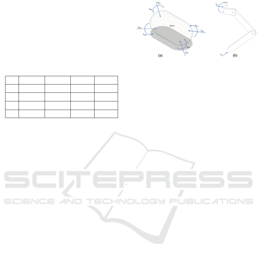
for forces and moments on each link. Fig. 2.a shows

the forces and moments exerted on the torso at all four

HFE joints, while Fig. 2.b illustrates the reaction

force and moment on a single leg at the HFE joint and

the ground.

The HFE joint reaction force and moment vectors,

𝐟

𝟏

𝒊𝒋

and 𝐧

𝟏

𝒊𝒋

are decomposed into two components:

one resulting from the leg's inertial forces and

moments, and the other from the ground reaction

forces, as shown below in (1) and (2), for a single leg.

𝒇

𝒃

𝟏

𝒇



𝒃

𝟏

𝒇



𝒃

𝟏

(1)

Figure 2: Schematic illustration of forces and moments

acting on the torso and a representative leg.

𝒏

𝒃

𝟏

𝒏



𝒃

𝟏

𝒏



𝒃

𝟏

(2)

where, 𝒇

𝒃

𝟏

and 𝒏

𝒃

𝟏

represents the reaction force and

moments exerted by link 1 on the body, excluding the

contribution from the ground reaction force, and

𝒇



𝒃

𝟏

𝑅





𝒇

𝟒

and 𝒏



𝒃

𝟏

𝑷

𝒃



𝑅





𝒇

𝟒

represents

the reaction forces and moments exerted by the legs

on the body due to ground reaction force.

All force and moment vectors here are expressed

in body-fixed reference frame.

In the initial stage, 𝒇



𝒃

𝟏

and 𝒏



𝒃

𝟏

are computed

under the assumption that all legs are suspended in

air, implying that 𝐟

𝟒

𝒊𝒋

and 𝐧

𝟒

𝒊𝒋

to be 0. The algorithm

then recursively propagates calculating forces and

moments through each joint, progressing toward the

HFE joint for each leg. In the second stage, the still

unknown ground reaction force and moment

components are determined by solving the dynamic

force and moment balance equations as shown in (3)

and (4).

∑

𝑅







𝒇

𝟒

𝟒,𝒊𝒋

𝑚



𝒂

𝒃

−𝑮

𝒃

−

∑

𝒇



𝒃

𝟏,𝒊𝒋

(3)

∑

𝑷

𝒃

𝟒,𝒊𝒋

𝑅







𝒇

𝟒

𝟒,𝒊𝒋

𝐼



𝜶

𝒃

−𝐼



𝝎

𝒃

𝝎

𝒃

−

∑

𝒏



𝒃

𝟏,𝒊𝒋

(4)

Equations (3) and (4) are formulated with known

right-hand side terms, while the unknowns are

grouped into left-hand side expressions involving

𝒇

𝟒

𝟒,𝒊𝒋

for the four legs. In-depth analyses of the

solution are presented in the subsequent sections.

The system's inverse dynamic analysis is carried

out using the recursive Newton-Euler algorithm

(Craig, 2005). Joint velocities and accelerations are

computed from the body frame to the foot frame using

an outward iteration process. Using these velocity and

acceleration vectors, the inertial force vector 𝑭

𝒊

and

inertial moment vector 𝑵

𝒊

acting on the ith link are

computed via the Newton-Euler equations. The

reaction force 𝑓



and reaction torque 𝑛



at the ith joint

are computed recursively using the reaction force and

torque vectors from the subsequent joint i+1, based

ICINCO 2025 - 22nd International Conference on Informatics in Control, Automation and Robotics

412

on the previously calculated force and moment

vectors.

The presented formulations are defined with

respect to a single leg and must therefore be applied

independently to all four legs. The recursive

computation initiates at the last link (Link 3), where

the ground reaction force is either evaluated or

assumed to be zero in the case of a non-contact

(swing) phase. A systematic approach for computing

the ground reaction forces is developed and will be

detailed in the subsequent section.

4 INVERSE DYNAMIC

SOLUTION

The inverse dynamics analysis, which involves

computing joint torques based on the specified

motion of the robot, including the robot’s body, is

conducted with respect to a specific set of ground

reaction forces. Depending on the gait pattern,

multiple leg support configurations are possible. The

nominal configuration corresponds to the quadruped

standing on all four legs, permitting body motions

such as roll, pitch, yaw, and vertical displacement. In

contrast, during a static walking gait, three legs

remain in contact with the ground at any given time,

while one leg is in the swing phase. In dynamic gaits

such as trotting or pacing, two diagonally or laterally

opposed legs are in contact with the ground at any

given time, while the remaining two are in the swing

phase. Additionally, there exist phases, such as during

jumping or bounding, where all four legs are airborne.

To compute the joint torques, required for rigid-body

dynamics, it is essential to determine the

corresponding ground reaction forces. The ground

reaction force computation for each of these scenarios

is discussed in in the following subsections.

Figure 3: Ground reaction force on the legs of quadruped

system.

4.1 Ground Support on Four Legs

When all four legs are in contact with the ground,

ground reaction forces act on each leg, as depicted in

Fig. 3. This configuration introduces twelve unknown

force components, represented as 𝑓

,





, where i

refers to the left or right leg and j indicates front or

rear leg. However, the dynamic equilibrium of the

robot's body yields only six equations, three for linear

forces and three for moments, corresponding to (3)

and (4). As the system contains six more unknowns

than available equations, it becomes statically

indeterminate and hence requires six additional

constraint equations to fully resolve the ground

reaction forces.

To address this issue, a set of simplifying

assumptions is introduced to provide the necessary

constraint equations. The vertical ground reaction

forces (Z-direction) for all four legs are treated as

independent, contributing four separate unknowns. In

contrast, the ground reaction forces in the X-direction

are assumed to be equal across all four legs, reducing

the associated unknowns to a single variable.

Likewise, the Y-direction ground reaction forces are

assumed identical for all legs, introducing only one

additional unknown. These assumptions reduce the

total number of unknowns to six, allowing the system

to be fully determined from the available dynamic

equilibrium equations.

4.2 Ground Support on Three Legs

During static walking, the robot maintains ground

contact with three legs, resulting in nine unknown

ground reaction force components, still exceeding the

number of available equilibrium equations. To

address this, the same assumptions applied in the full

support case are maintained for the Z and X

directions: three independent vertical (Z-axis)

reaction forces and one common reaction force along

the X-axis, reducing the number of unknowns in these

directions to four. However, the reaction force

components along the Y-direction are viewed as

follows. When one leg is lifted, it is assumed that the

leg on the same side experiences a distinct reaction

force component from the ground along the Y than

the two legs on the opposite side, which are assumed

to receive equal lateral reaction force components

from the ground. This introduces two additional

unknowns along the Y-axis. With these assumptions,

the total number of unknowns is reduced to six,

matching the number of dynamic equilibrium

equations and allowing the reaction forces to be

determined. The static condition in these scenarios

Kinematic and Dynamic Analysis of Quadruped Legged Robots: A New Formulation Approach

413

justifies the simplifying assumptions used. In

dynamic walking, however, all ground reaction force

components are treated independently as outlined next.

4.3 Ground Support on Two Legs and

During Airborne

In dynamic gaits such as trot and pace, the robot

maintains ground contact with only two legs at any

given time. Under these conditions, the reaction force

problem becomes more tractable, as the system

involves only six unknown ground reaction force

components, three per contact point, which can be

determined directly from the equations of motion

without necessitating additional assumptions or

constraints.

Conversely, during a pronk gait, the robot enters

an aerial phase wherein all limbs are off the ground,

resulting in zero ground contact. Consequently, the

ground reaction forces at the feet are identically zero.

This absence of external contact forces simplifies the

system dynamics, allowing for direct computation of

the internal reaction forces and moments exerted by

the legs on the robot’s body based solely on its inertial

properties and joint torques.

5 FORWARD DYNAMICS

With the forward dynamic formulation, the objective

is to determine the acceleration components

corresponding to the generalized coordinates

assuming the knowledge of the input torque vector.

The focus of this study is on two different gait

patterns, namely the static walking gait and the

dynamic trotting gait.

In the case of a static walking gait, three legs

maintain ground contact at any instant of time. This

statically stable support configuration allows the

estimation of the robot body's pose through the

known joint angles of the supporting legs. Under the

assumption of static equilibrium and using forward

kinematic relations, the system is described by twelve

generalized coordinates, corresponding to the three

joint angles 𝜃

,

, 𝜃

,

, 𝜃

,

 for each of the four legs,

resulting in a total of twelve joint coordinates. On the

other hand, during the dynamic trotting gait, only two

diagonally opposed legs are in contact with the

ground at any given moment, which results in a

reducing the support polygon to a line. The associated

body rotation cannot be determined solely from the

displacement of the attachment points of the two

supporting legs. To address this limitation, the roll

angle ∅ of the quadruped system is introduced as an

additional generalized coordinate, increasing the total

number of generalized coordinates to thirteen.

The accelerations of the generalized coordinates,

twelve in the case of the static walking gait and

thirteen in the case of the dynamic trotting gait, are

obtained through the forward dynamics formulation.

The resulting accelerations are numerically integrated

twice to obtain the joint velocities and displacements.

The body’s orientation and angular rates are

subsequently determined through forward

kinematics, as described in the previous section. To

evaluate the dynamic model, the inverse dynamics

formulation based on the Newton-Euler recursive

algorithm is used to numerically compute the

system’s inertia matrix, as well as the gravity,

Coriolis, and centrifugal torque vectors (Harib &

Srinivasan, 2003; Walker & Orin, 1982).

Once the inertia matrix, Coriolis and centrifugal

torque vector, and gravity torque vector have been

computed, they are combined with the input torque

vector, generated by the control law, to solve for the

joint acceleration vector as shown in (5). This

acceleration vector is then numerically integrated

twice to obtain the joint velocity and displacement

vectors.

𝒒



= 𝑀



𝒒







𝝉−𝑪



𝒒, 𝒒





−𝑮(𝒒)

)

(5)

A comprehensive analysis of the system dynamics,

control implementation, and experimental validation

are presented in (Sureshkumar, 2025).

6 SIMULATION RESULTS

A simulation was conducted in Simulink to validate

the proposed dynamic formulation. This section

presents a brief overview of the open-loop control

results, wherein the acceleration, velocity, and

displacement vectors obtained from the forward

dynamics are compared against the corresponding

vectors derived from the desired trajectory, computed

using inverse kinematics.

Fig. 4, illustrates the path planning profile for the

dynamic trotting gait, depicting the positional

trajectories of both the robot’s body and the end-

effectors (feet) over the course of the gait cycle. These

trajectories serve as essential inputs for the inverse

kinematics computation, which subsequently yields

the desired joint angle trajectories required to achieve

the planned motion. For the dynamic trotting gait, as

depicted in Figure 5.7, the back-right (BR) and front-

left (FL) legs move in unison during one step phase,

followed by the back-left (BL) and front-right (FR)

ICINCO 2025 - 22nd International Conference on Informatics in Control, Automation and Robotics

414

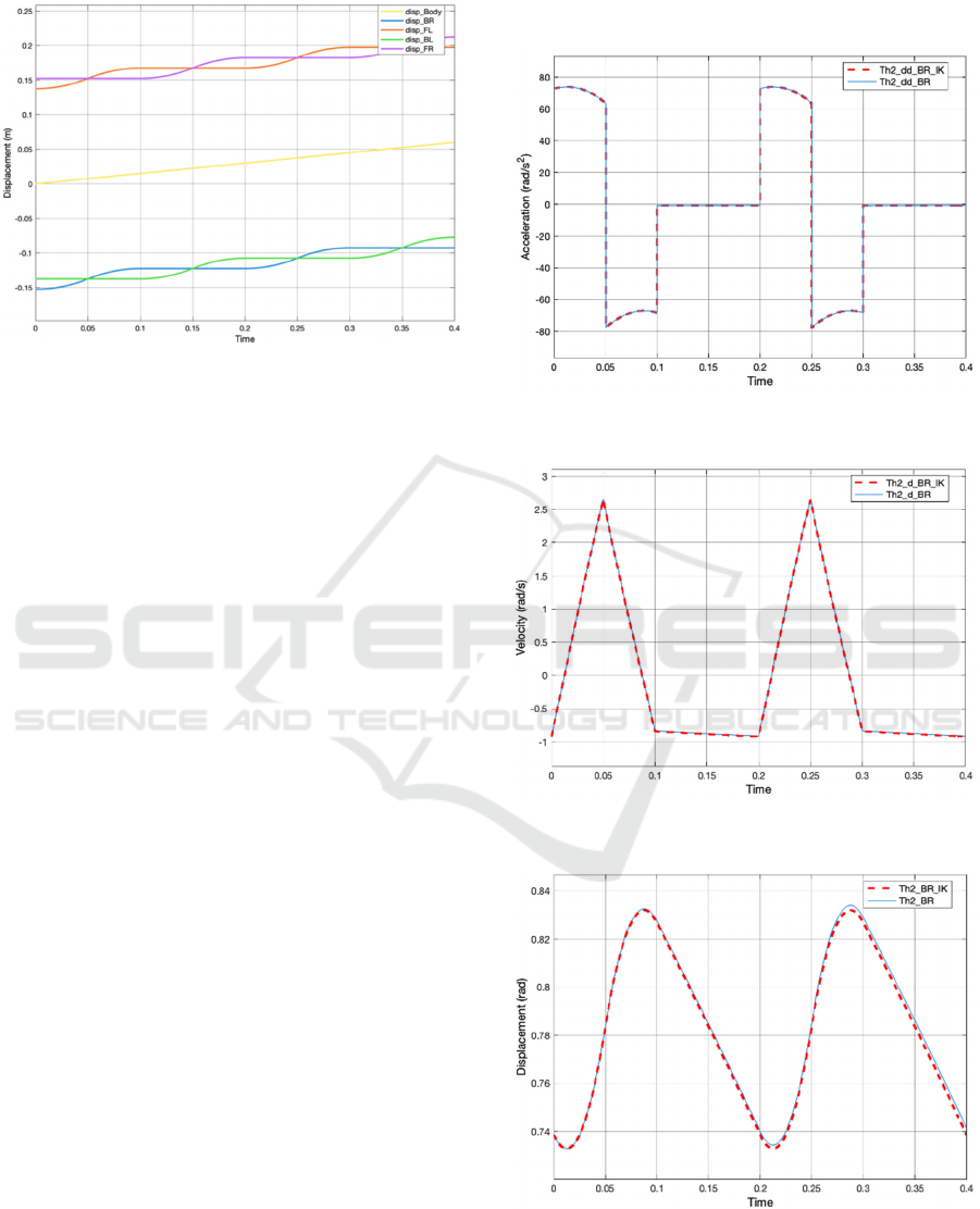
legs during the subsequent phase.

Figure 4: Gait profile for dynamic trotting.

Initially, the inverse kinematics is used to

compute joint positions, velocities, and accelerations,

which serve as inputs to the inverse dynamics model

for calculating the required joint torques. As

discussed in the previous section, the inertia matrix,

Coriolis and centrifugal torque vector, and

gravitational torque vector are determined

numerically. These, along with the input torque

vector, are then used in the forward dynamics

formulation to solve for joint accelerations as

described in (5). The computed joint accelerations are

subsequently integrated twice over time to obtain the

corresponding joint velocities and displacements. The

resulting joint kinematic trajectories are then

compared against those derived from the inverse

kinematics to validate the proposed methodology.

The comparison results in the form of acceleration,

velocity and displacement of the HFE joints of the

back-right leg are shown in Fig. 5 – 7.

Figure 5-7 illustrates high agreement of the

simulation of the joint trajectories obtained from the

forward dynamic simulation with those computed via

the inverse kinematics based on the desired trajectory.

The observed discrepancies are minimal, with a

maximum percentage error of only 0.0006%.

Such results indicate strong validation for the

accuracy and effectiveness of the proposed

methodology in modelling the system dynamics. The

close agreement between the forward dynamics

outputs and the reference trajectories derived from

inverse kinematics demonstrates the reliability of the

implemented numerical framework. Additionally, the

consistency across results confirms the correctness of

the developed code and simulation environment,

ensuring its proper functionality for dynamic

analysis. This validation reinforces the robustness of

the computational framework and supports its

applicability to real-world quadruped robotic systems

for dynamic modelling and control.

Figure 5: Comparison of the HFE joint acceleration for the

back-right (BR) leg.

Figure 6: Comparison of the HFE joint velocity for the

back-right (BR) leg.

Figure 7: Comparison of the HFE joint displacement for the

back-right (BR) leg.

Kinematic and Dynamic Analysis of Quadruped Legged Robots: A New Formulation Approach

415

7 CONCLUSIONS

This study presents the development of a novel

framework for formulating the system dynamics of a

quadruped robot through the systematic selection of

kinematic and dynamic constraints. The dynamic

model is constructed using the recursive Newton-

Euler formulation to ensure computational efficiency.

The forward dynamics is implemented by deriving

the joint acceleration vector from the system rigid

body dynamic equation. A numerical approach is

used to compute the inertia matrix, Coriolis and

centrifugal torque vector, and gravitational torque

vector. These dynamic terms are then utilized to solve

for the joint acceleration vector which could be then

integrated twice in the simulation to obtain the joint

velocity and displacement vectors.

A simulation environment was established for a

quadruped system comprising twelve actuators, with

each leg driven by three independently actuated

joints, enabling full mobility and control authority.

Motion trajectories were generated based on a

predefined dynamic trotting gait. The accuracy of the

dynamic formulation and the developed simulation

model was validated by simulating the system under

representative trajectories corresponding to dynamic

trotting gaits.

A comprehensive analysis of the dynamic

formulation, with a particular focus on the forward

dynamics could include closed-loop control

simulations employing a feedforward and feedback

control strategies, followed by experimental

validation to assess the accuracy and effectiveness of

the proposed approach.

ACKNOWLEDGEMENT

This research is supported by NSSTC UAE-

University under Grant No. 12R153.

REFERENCES

Bennani, M., & Giri, F. (1996). Dynamic modelling of a

four-legged robot. Journal of Intelligent and Robotic

Systems, 17, 419-428.

Craig, J. J. (2005). Introduction to Robotics: Mechanics and

Control. Pearson/ Prentice Hall. https://books.google

.ae/books?id=ZJkOSgAACAAJ

Fu, J., & Gao, F. (2022). Dynamic stability analyzes for a

parallel–serial legged quadruped robot. International

Journal of Advanced Robotic Systems, 19(5),

17298806221132081.

Harib, K., & Srinivasan, K. (2003). Kinematic and dynamic

analysis of Stewart platform-based machine tool

structures. Robotica, 21(5), 541-554.

He, Y., Guo, S., Shi, L., Pan, S., & Guo, P. (2016). Dynamic

gait analysis of a multi-functional robot with bionic

springy legs. 2016 IEEE International Conference on

Mechatronics and Automation,

Liu, M., Qu, D., Xu, F., Zou, F., Di, P., & Tang, C. (2019).

Quadrupedal robots whole-body motion control based

on centroidal momentum dynamics. Applied Sciences,

9(7), 1335.

Morais, S., Singh, H., & Acharya, A. (2021). Trajectory and

Gait Planning of a Quadruped using Adams and

Simulink. 2021 4th Biennial International Conference

on Nascent Technologies in Engineering (ICNTE),

Potts, A., Cruz, D., & Gacovski, Z. (2011). A Kinematical

and Dynamical Analysis of a Quadruped Robot. Mobile

Robots–Current Trends, 239-262.

Shi, Y., Li, S., Guo, M., Yang, Y., Xia, D., & Luo, X.

(2021). Structural design, simulation and experiment of

quadruped robot. Applied Sciences, 11(22), 10705.

Sun, L., Zhou, Y., Chen, W., Liang, H., & Mei, T. (2007).

Modeling and robust control of quadruped robot. 2007

International Conference on Information Acquisition,

Sureshkumar, V. (2025). Dynamic analysis and control of a

quadruped robotic system based on Newton-Euler

formulation [PhD Thesis, United Arab Emirates

University]. Al Ain - UAE.

Walker, M. W., & Orin, D. E. (1982). Efficient dynamic

computer simulation of robotic mechanisms.

ICINCO 2025 - 22nd International Conference on Informatics in Control, Automation and Robotics

416