Redundancy Resolution in Multiple Feasibility Maps via MultiFM-RRT
Marc Fabregat-Ja
´
en
1 a
, Adri
´
an Peidr
´
o
1 b
, Mar
´
ıa Flores
1 c
, Luis Pay
´
a
1,2 d
and
´
Oscar Reinoso
1,2 e
1
Instituto de Investigaci
´
on en Ingenier
´
ıa de Elche, Universidad Miguel Hern
´
andez, Avda. Universidad s/n, Elche, Spain
2
ValgrAI: Valencian Graduate School and Research Network of Artificial Intelligence, Cam
´
ı de Vera s/n, Valencia, Spain
fl
Keywords:
Redundancy Resolution, RRT, MultiFM-RRT, Feasibility Maps, Redundant Manipulators.
Abstract:
This paper presents MultiFM-RRT, a novel algorithm for redundancy resolution in kinematically redundant
manipulators based on the exploration of multiple Feasibility Maps (FMs). They encode all valid config-
urations of redundant variables for a prescribed task trajectory, enabling global optimization and constraint
satisfaction. Unlike traditional velocity-based methods, which are limited to local solutions, and grid-based
methods, which are computationally intensive, MultiFM-RRT leverages the Rapidly-exploring Random Tree
(RRT) framework to efficiently explore the space of feasible solutions across multiple feasibility maps. The al-
gorithm incorporates singularity maps to enable transitions between different aspects, ensuring comprehensive
coverage of the solution space. By computing feasibility maps online and guiding exploration with probabilis-
tic sampling of goal and singularity sets, MultiFM-RRT achieves a balance between computational efficiency
and global optimality. The proposed approach is demonstrated on a Stewart parallel platform, illustrating its
ability to generate feasible, constraint-satisfying trajectories while efficiently handling redundancy.
1 INTRODUCTION
Kinematically redundant robots are characterized by
having more degrees of freedom (DoF) n than the di-
mension m of the main or primary task they are re-
quired to perform. For instance, a planar manipu-
lator with three joints (3-DoF) that must control the
end-effector position (p
x
, p
y
) in the plane exhibits one
degree of redundancy (r = 1), since only two DoF
are necessary for this task. This surplus of DoF en-
hances the manipulator’s versatility, as it can be ex-
ploited to fulfill additional secondary objectives or
constraints, such as minimizing joint torques or en-
ergy, or avoiding singularities and obstacles (Peidro
and Haug, 2023). However, this flexibility comes
at the cost of increased computational complexity:
the inverse kinematics problem (IKP) (i.e, determin-
ing the joint displacements required to achieve a de-
sired end-effector position) admits infinitely many so-
lutions. The challenge of selecting a suitable solution
from this infinite set is known as the redundancy res-
olution problem.
a
https://orcid.org/0009-0002-4327-0900
b
https://orcid.org/0000-0002-4565-496X
c
https://orcid.org/0000-0003-1117-0868
d
https://orcid.org/0000-0002-3045-4316
e
https://orcid.org/0000-0002-1065-8944
In practice, redundancy resolution is typically ad-
dressed for a prescribed trajectory of the task vari-
ables. Given a desired task trajectory x(t), 0 < t < t
g
,
a redundancy resolution algorithm must generate the
time evolution q(t) of all n joint coordinates, taking
into account the infinite solution set at each instant
and any imposed constraints or secondary objectives.
Approaches to this problem are generally classified as
either velocity-based or position-based.
Velocity-based methods rely on the differential re-
lationship
˙
x = J
˙
q, where J is the non-square m × n
Jacobian matrix. These methods, including pseu-
doinverse and optimization-based techniques, com-
pute joint velocities
˙
q and then integrate them. Pseu-
doinverse approaches (Whitney, 1969) yield
˙
q = J
†
˙
x
plus a nullspace term for optimizing secondary crite-
ria (Kazemipour et al., 2022), with J
†
denoting the
Moore-Penrose pseudoinverse. Optimization-based
methods formulate a minimization problem for
˙
q,
subject to the equality constraint
˙
x = J
˙
q, thus avoid-
ing explicit inversion (Zanchettin and Rocco, 2017).
The main strengths of velocity-based methods are
their simplicity and suitability for real-time control.
However, they are typically limited to locally optimal
solutions, may encounter issues with non-holonomy
and singularities (when using the pseudoinverse), and
can struggle to enforce constraints that are more natu-
158
Fabregat-Jaén, M., Peidró, A., Flores, M., Payá, L. and Reinoso, Ó.
Redundancy Resolution in Multiple Feasibility Maps via MultiFM-RRT.
DOI: 10.5220/0013835700003982
Paper published under CC license (CC BY-NC-ND 4.0)
In Proceedings of the 22nd International Conference on Informatics in Control, Automation and Robotics (ICINCO 2025) - Volume 2, pages 158-165
ISBN: 978-989-758-770-2; ISSN: 2184-2809
Proceedings Copyright © 2025 by SCITEPRESS – Science and Technology Publications, Lda.

rally expressed at the position level, such as collision
avoidance (Peidro and Haug, 2023).
Position-based methods address these limitations
by working directly at the configuration level. Here,
redundancy resolution involves identifying all sets of
joint coordinates q that achieve a given task value x.
These solution sets are, in general, manifolds known
as self-motion manifolds (Burdick, 1989). By ex-
ploring all self-motion manifolds for a given x, one
can identify the configuration q
∗
that globally op-
timizes secondary objectives, enabling globally op-
timal redundancy resolution (Fabregat-Ja
´
en et al.,
2025). This approach, however, is computationally
demanding, as the computation of self-motion mani-
folds is nontrivial (Albu-Sch
¨
affer and Sachtler, 2023).
A related strategy is provided by Feasibility Maps
(FMs) (Wenger et al., 1993; Reveles et al., 2016),
which represent all feasible values of a set of r redun-
dant variables at each instant t along the trajectory.
FMs facilitate trajectory planning in the space of re-
dundant variables, allowing for the avoidance of ob-
stacles and singularities while optimizing additional
criteria.
Several researchers have proposed the use of FMs
to address the redundancy resolution problem. For
example, (P
´
amanes G et al., 2002) proposed using
FMs to plan collision-free trajectories while mini-
mizing the change in the free parameter. More re-
cently, (Ferrentino and Chiacchio, 2020) presented
a method to globally solve the redundancy resolu-
tion problem by performing an exhaustive grid search
across all FMs, which is computationally expensive.
In contrast, (Fabregat-Jaen et al., 2023) proposed a
more time-efficient approach based on the Rapidly-
exploring Random Tree (RRT) algorithm. In their
method, only the FM corresponding to the initial con-
figuration is explored, and the FM is computed on-
the-fly as the algorithm progresses, eliminating the
need for precomputation. In (Fabregat-Ja
´
en et al.,
2024), the concept of FMs was extended to include
the notion of augmented feasibility maps, which in-
corporate the task dimension x into the FM space,
allowing for simultaneous path planning and redun-
dancy resolution.
In this paper, we introduce MultiFM-RRT, a novel
algorithm that aims to strike a balance between the
two aforementioned approaches. Similar to (Fer-
rentino and Chiacchio, 2020), MultiFM-RRT ex-
plores all FMs, but it does so more efficiently by lever-
aging the RRT algorithm. Additionally, it computes
the FMs online, as in (Fabregat-Jaen et al., 2023),
thereby avoiding the need for precomputation and im-
proving computational efficiency.
The rest of the paper is organized as follows.
Section 2 introduces the concept of feasibility maps
and important related concepts. Section 3 presents
the MultiFM-RRT algorithm, which extends the RRT
framework to explore multiple feasibility maps simul-
taneously. Section 4 provides an example of the al-
gorithm in action, and Section 5 concludes the paper
with a summary of the contributions and future work.
2 FEASIBILITY MAPS
2.1 Inverse Kinematics Problem
Equation (1) defines the constraint that relates the
joint space q ∈ R
n
and the task space x ∈ R
m
:
F(x, q) = 0
m×1
(1)
The IKP entails finding a joint configuration q that
satisfies Equation (1) for a given task-space point x.
However, even for non-redundant robots (where n =
m), the IK mapping is multi-valued in general. This
means that there exist multiple joint-space points q
that yield the same workspace point x.
To better understand this property, the concept
of aspects is introduced. As defined by (Borrel and
Li
´
egeois, 1986), aspects are connected sets of joint-
space points where the Jacobian matrix J(x, q) =
∂F
∂q
(hereafter J) mantains full rank m. In other words,
aspects define subsets of the joint space where singu-
larities do not exist. Following this definition, it is
directly derived that transitions between aspects are
marked by singularities, at which point J loses rank.
The multi-valuedness of the IK is exacerbated for
redundant manipulators, where the IKP becomes un-
derdetermined: as n > m, there are more unknowns
than equations from which to solve the IKP. When re-
dundancy arises, the degree of redundancy r is defined
as the difference between the dimensionality of joint
and task spaces: r = n −m.
2.2 Task Space Augmentation
When kinematic redundancy arises, by fixing r so-
called free parameters to known values, the IKP be-
comes determined, and a unique solution can be found
for each aspect. Note that the free parameters can be
chosen arbitrarily, as long as they are a differentiable
function of the joint space coordinates q, and inde-
pendent of the task space coordinates x. However,
in most cases, the best selection of free parameters is
simply r joint variables to which values are freely as-
signed. For simplicity, for the rest of the paper, we
will consider this case, and refer to the free parame-
ters as q
r
∈ R
r
, where q
r
consists of r components of
Redundancy Resolution in Multiple Feasibility Maps via MultiFM-RRT
159

q. This addition of free parameters allows us to define
an augmented task space x
a
= (x, q
r
) ∈ R
m+r
.
In (P
´
amanes G et al., 2002), the consequences of
introducing the free parameters q
r
are analyzed. It is
shown that the newly introduced rows in J give rise
to additional singularities that are not present in the
original Jacobian. As a result, new sets of aspects, re-
ferred to as extended aspects, are produced. This im-
plies that, depending on the selection of q
r
, the num-
ber of extended aspects can vary.
The introduction of the augmented task space en-
ables the definition of a unique inverse kinematics
function, denoted as g(·). This function maps each
point in the augmented task space to a unique joint
configuration within a specific extended aspect:
q = g(x, q
r
, a) (2)
where a is determines the specific extended aspect to
which the returned joint configuration q belongs.
2.3 Feasibility Maps
Rather than treating the IKP as a pointwise problem,
it is often formulated as the tracking of a continuous
task. In this context, the objective is to find a contin-
uous path q(t) in the joint space that follows a given
trajectory x(t) in the task space. This trajectory is
typically parameterized by an arc-length parameter t,
which, for simplicity, we refer to as time. With this
parametrization, once the task trajectory is specified,
the task dimension m can effectively be reduced to
1, since the corresponding task space point x at any
given time t is obtained by evaluating x(t). The con-
cept presented next builds upon this idea.
According to (Wenger et al., 1993), the concept of
feasibility maps (FMs) represents the set of all joint
configurations q that satisfy the IKP for a given task
trajectory x(t) and a selection of free parameters q
r
,
in an r + 1 dimensional space. For each possible se-
lection of the extended aspect a, there exists a corre-
sponding FM. Formally, for each a, the FM is defined
as the connected set of points in the (t, q
r
) space that,
when solving the IKP via Equation (2) for the given
a, yield a valid joint configuration q:
F M
a
=

t
q
r




q = g(x(t), q
r
, a), q ∈ Q

(3)
where Q denotes the set of valid joint configura-
tions. The domain of Q is determined by the robot’s
kinematic constraints, as well as any additional task-
imposed constraints (e.g., joint limits, collision avoid-
ance, etc.).
Figure 1 shows the feasibility maps for a 2-
DoF planar manipulator represented in Figure 2.
The robot’s end effector is tasked with following a
parabolic trajectory in the y axis: x(t) = p
y
(t) =
−6.662t
2
+ 8.162t − 1.5 with t ∈ [0, 1], while avoid-
ing an ellipical obstacle. Joints are enforced to re-
main within the limits q
i
∈ [−π, π] for i = 1, 2. Hav-
ing r = 1, a single free parameter is selected, which
corresponds to the first joint variable q
1
. The inverse
kinematics function g(·) for this case is:
q =

q
1
π
2
+ σ(a)

π
2
− arcsin(p
y
(t) − sin q
1
)

− q
1

(4)
where σ(a) = ±1 is a sign function that determines
the resolution of the second joint variable q
2
based on
the extended aspect a.
FMs in Figure 1 are computed by sweeping plane
(t, q
1
) between its ranges (t ∈ [0, 1] and q
1
∈ [−π, π])
with a given discretization step. For each point (t, q
1
),
q is computed using Equation (4). If the evaluation
of a point results in non-real values (e.g., |p
y
(t) −
sinq
1
| > 1), the point is coloured purple. Similarly,
if the point results in a joint configuration that col-
lides with the environment, it is coloured red. Finally,
if the point results in a joint configuration that violates
the joint limits, it is coloured yellow. The remaining
points, which are left uncoloured, represent feasible
joint configurations, and conform the actual FM for
the given extended aspect a.
2.4 Singularity Maps
(Wenger et al., 1993) introduced the concept of singu-
larity maps (SMs), which represent the set of all sin-
gular points in the (t, q
r
) space that lie at the bound-
aries between different aspects. SMs are adjacent to
feasibility maps (FMs) and serve as gateways through
which the robot can transition from one FM to another
by passing through a singularity.
To compute the SMs, the time parameter t is
swept, and for each t, the values of the free param-
eters q
r
that produce singularities are determined.
Specifically, for the recurring example, singularities
occur when |p
y
(t)− sin q
1
| = 1, which corresponds to
the boundary of the domain of the arcsin function in
Equation (4). These SMs are shown in orange in Fig-
ure 1.
3 MULTIFM-RRT
The MultiFM-RRT algorithm proposed in this paper
extends the original RRT framework to enable the si-
multaneous exploration of multiple feasibility maps
(FMs). Algorithm 1 summarizes the main steps of
ICINCO 2025 - 22nd International Conference on Informatics in Control, Automation and Robotics
160

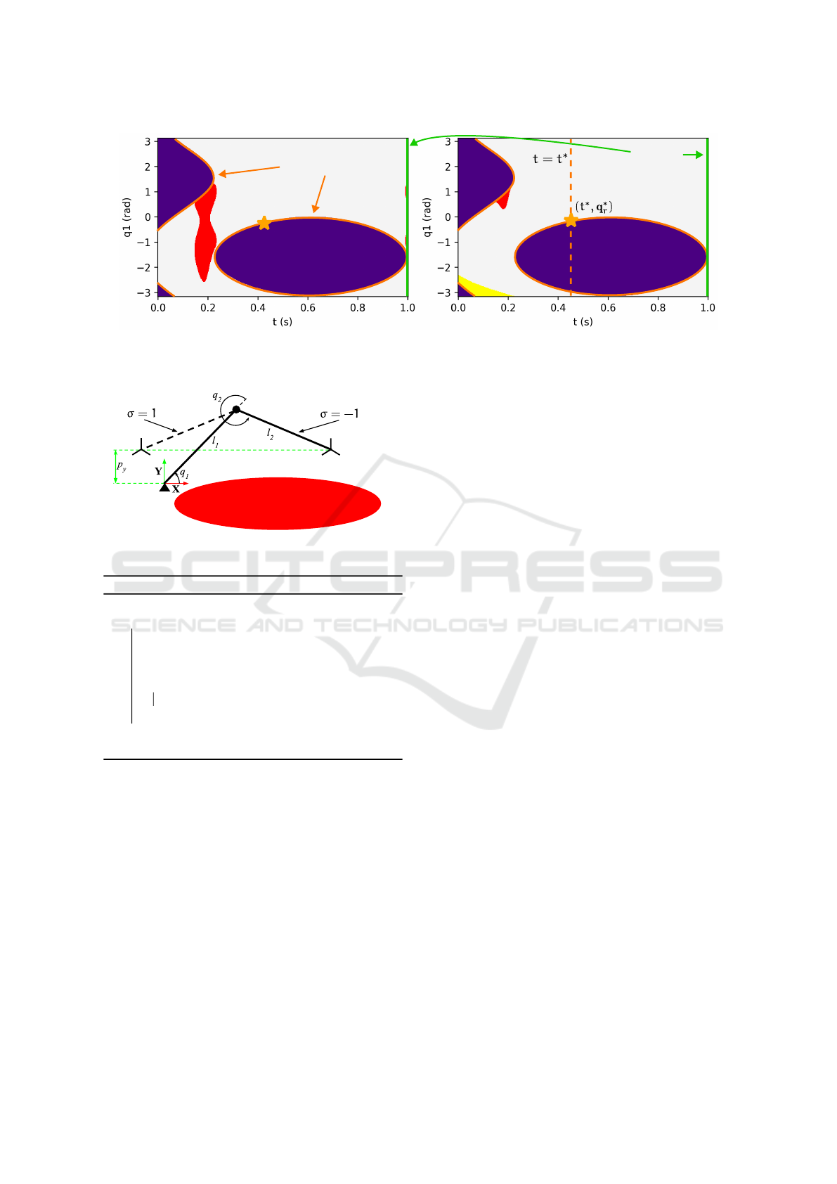
(a)
(b)
Singularity Maps
Goal set
Figure 1: Feasibility maps for a 2-DoF planar manipulator. (a) FM for the first extended aspect (σ = 1). (b) FM for the second
extended aspect (σ = −1). Colour regions indicate sets of invalid joint configurations: red for collisions, yellow for joint
limits, and purple for complex solutions. Singularity maps are shown in orange, and goal sets are shown in green.
Figure 2: 2-DoF planar manipulator tasked with task x = p
y
.
Algorithm 1: MultiFM-RRT algorithm.
Initialize tree T with root node n
0
= s
0
for i = 1, 2, . . . , i
max
s
random
← SAMPLESTATE(α, β)
n
near
← NEARESTNODE(s
random
, T )
n
new
← STEER(n
near
, s
random
, ∆s)
if FEASIBLECONNECTION(n
near
, n
new
)
Add n
new
to T with parent n
near
end
end
P ← BESTPATH(T , c(·))
MultiFM-RRT. While the overall structure remains
similar to the standard RRT, the key differences lie
in the adaptation of specific procedures to accommo-
date the characteristics of FMs and the requirements
of multi-map exploration.
First, the algorithm initializes a tree T with a root
node n
0
(without parent) representing the initial state
s
0
of the robot. A state s = [t, q
T
r
, a] is defined as a
point in the space (t, q
r
) of a specific F M
a
. Remem-
ber that, given a state s, the corresponding joint con-
figuration q can be directly obtained by solving the
IKP using Equation (2). A node n is a state s that has
been added to the tree T with an associated parent,
and is defined as a pair n = (s, n
parent
), where n
parent
is the parent node of n in the tree.
The algorithm then enters its main loop, which
runs for up to i
max
iterations. This value sets an upper
limit on the number of nodes that can be added to the
tree T ; however, the actual number of nodes will typ-
ically be less, since many sampled states may be in-
feasible and therefore not included. In Section 4, we
analyze how varying i
max
influences the algorithm’s
performance and solution quality.
At each iteration, the algorithm samples a ran-
dom state s
random
from the FM space using the SAM-
PLESTATE procedure. By default, this procedure gen-
erates a random point in the (t, q
r
) space of a ran-
domly selected feasibility map F M
a
, with the ex-
tended aspect a chosen uniformly at random. In addi-
tion, two parameters, α and β, control the probability
of sampling from specialized subsets: the goal set and
the singularity maps (SMs), respectively. These prob-
abilites are usually kept low, e.g., α = β = 0.05 (5%).
The goal set, sampled with probability α, consists
of all states s = [t, q
T
r
, a] for which the task trajectory
x(t) is completed, i.e., t = t
goal
, where t
goal
denotes
the final time of the trajectory. In Figure 1, the goal
set is represented by the green vertical lines at t =
1, which correspond to the end of the task trajectory.
The goal set is used to guide the exploration towards
the completion of the task.
Conversely, with probability β, the algorithm sam-
ples from the SMs: it selects a random time t
∗
, com-
putes the intersections q
∗
r
between the hyperplane
t = t
∗
and the SMs, and randomly selects one of these
intersections, such that (t
∗
, q
∗
r
) corresponds to a sin-
gularity, as defined in Section 2.4, and illustrated in
Figure 1. Note that, by definition, singular points do
not belong to any aspect, since they form the bound-
aries between aspects. As a result, a sampled state
s
random
from the SMs will not be associated with a
valid extended aspect a. This property, and sampling
Redundancy Resolution in Multiple Feasibility Maps via MultiFM-RRT
161

probability, is later leveraged to enable transitions be-
tween different FMs.
After sampling a state s
random
, the algorithm iden-
tifies the nearest node n
near
in the tree T using the
NEARESTNODE procedure. This procedure performs
a nearest-neighbor search according to a user-defined
cost function c(·), which, for simplicity, we have cho-
sen as the Euclidean distance in the (t, q
r
) space. Cru-
cially, the search is restricted to two particular condi-
tions:
1. The nearest node n
near
must belong to the same
FM as the sampled state s
random
, i.e., a
near
=
a
random
. However, this condition is relaxed when
either s
random
or n
near
belong to the SMs (i.e. have
no defined aspect), in which case this condition is
ignored.
2. The nearest node n
near
must have a time value
t
near
< t
random
, ensuring that the time parameter
t remains monotonically increasing. This con-
straint ensures the completion of the task trajec-
tory x(t) and prevents the algorithm from gener-
ating solutions that move backward in time.
Once the nearest node n
near
is identified, the
algorithm generates a new node n
new
by steering
from n
near
toward the sampled state s
random
using the
STEER procedure. This procedure produces a new
state s
new
at a fixed distance ∆s from n
near
towards
s
random
, controlling the resolution of the exploration.
The assignment of the aspect a
new
for n
new
depends
on whether either state is associated with a SM (i.e.,
has no defined aspect):
1. If s
random
belongs to the SMs, then n
new
inherits
the aspect of n
near
(a
new
= a
near
), unless s
random
is within ∆s of n
near
, in which case n
new
is set to
s
random
with undefined aspect.
2. If n
near
belongs to the SMs, then n
new
inherits the
aspect of s
random
(a
new
= a
random
).
Finally, the algorithm checks whether the connec-
tion between n
near
and n
new
is feasible using the FEA-
SIBLECONNECTION procedure. This procedure veri-
fies that the path from n
near
to n
new
lies entirely within
a FM, i.e., it does not cross complex-solution regions.
This check is performed by discretizing the path using
a given resolution ∆ f and evaluating the feasibility of
each point along the path. Additionally, it checks that
the path does not violate any additional constraints,
such as joint limits or collisions. If the connection is
feasible, the new node n
new
is added to the tree T with
n
near
as its parent.
Once the tree T has been constructed by exhaust-
ing the maximum number of iterations i
max
, the al-
gorithm computes the best path P using the BEST-
PATH procedure. This procedure evaluates every path
that joins the root node n
0
to a node n
goal
that be-
longs to the goal set, and selects the path with the
lowest cost according to the user-defined cost func-
tion c(·). The resulting path P is a continuous trajec-
tory in the joint space that satisfies the task trajectory
x(t), since the time parameter t is monotonically in-
creasing, reaches t
goal
, and the path does not traverse
infeasible regions. Note that the returned path P is
polygonal due to the nature of the RRT algorithm.
The smoothing of the path can be performed using
any standard path smoothing technique, such as the
one presented in (Fabregat-Ja
´
en et al., 2024).
4 EXAMPLE
4.1 Application to a Stewart Platform
This section illustrates the application of the
MultiFM-RRT algorithm to a Stewart platform. The
considered Stewart platform, depicted in Figure 3,
features a double-ring configuration: its six UPS
(Universal-Prismatic-Spherical) linear actuators with
lengths q
1
, q
2
, . . . , q
6
are arranged in two concentric
rings, each containing three actuators. The positions
of the universal joints with respect to the fixed base
center W are denoted a
j
and are listed in Table 1. Sim-
ilarly, the positions of the spherical joints relative to
the mobile platform center Σ are given by b
j
in Table
1. The pose of the mobile platform is described by
p = (x,y, z, α, β, γ), where (x, y, z) specifies the posi-
tion of Σ with respect to W , and (α, β, γ) are the XYZ
Euler angles defining the platform’s orientation rela-
tive to the base. The relationship between the joint
coordinates q and the platform pose p is:
∥R(α, β, γ)b
j
+ [x, y, z]
T
− a
j
∥
2
− q
2
j
= 0, j = 1, . . . , 6
(5)
where R(α, β, γ) is the rotation matrix corresponding
to the XYZ Euler angles (α, β, γ).
The robot is required to follow an arc-shaped tra-
jectory in the (X,Y ) plane, simulating a machining
operation with a cutting tool along the Z axis of the
mobile platform. Note that, since the cutting tool is
rotating along the Z axis, the Euler angle γ is not rel-
evant for this task, and the robot becomes kinemat-
ically redundant, where the objective is to track the
following task trajectory:
x(t) =





x
y
z
α
β





=





cos(t)
sin(t)
0.8
0
0





, t ∈ [0, 0.8] (6)
ICINCO 2025 - 22nd International Conference on Informatics in Control, Automation and Robotics
162

Table 1: Joint positions of the double-ring Stewart platform.
Joint j a
j
b
j
1


0.6cos(0)
0.6sin(0)
0.05




0.6cos(0)
0.6sin(0)
−0.05


2


0.4cos(0)
0.4sin(0)
0.05




0.4cos(180
◦
)
0.4sin(180
◦
)
−0.05


3


0.6cos(120
◦
)
0.6sin(120
◦
)
0.05




0.6cos(120
◦
)
0.6sin(120
◦
)
−0.05


4


0.4cos(120
◦
)
0.4sin(120
◦
)
0.05




0.4cos(300
◦
)
0.4sin(300
◦
)
−0.05


5


0.6cos(−120
◦
)
0.6sin(−120
◦
)
0.05




0.6cos(−120
◦
)
0.6sin(−120
◦
)
−0.05


6


0.4cos(−120
◦
)
0.4sin(−120
◦
)
0.05




0.4cos(−300
◦
)
0.4sin(−300
◦
)
−0.05


An additional kinematic constraint is imposed on
the robot: collisions between the linear actuators are
prevented by ensuring that the distance between ev-
ery pair of actuators remains greater than a minimum
threshold, d
min
= 4 cm. The length of the first linear
actuator, q
1
, is chosen as the free parameter, q
r
= [q
1
],
and is restricted to the interval [0.75, 1.75] m. With
this selection of free parameter, the robot presents two
FMs, corresponding to the two extended aspects a,
which result from the two possible resolutions of γ
W
X
Y
Z
Z
X
Y
Cutting tool
U
S
P
Σ
𝑞
𝑖
Fixed base
Mobile platform
𝐚
𝑖
𝐛
𝑖
(a)
Figure 3: Double-ring Stewart platform with six UPS linear
actuators.
from Equation (5) for i = 1 and for the given values
of x(t) (Peidro et al., 2018).
The MultiFM-RRT parameters are set as follows:
the maximum number of iterations is i
max
= 2000; the
steering step size is ∆s = 0.5 cm; the singularity and
goal sampling biases are α = β = 0.05; and the path
discretization resolution for feasibility checks is ∆ f =
0.02.
Figure 4 displays the FMs computed for the Stew-
art platform during task execution. The same color
scheme as in Figure 1 is applied. It is important to
note that FMs are not precomputed, but are generated
online as the algorithm progresses; they are shown
here solely for illustration.
Figure 4 also depicts the tree T produced by a rep-
resentative run of the MultiFM-RRT algorithm. The
initial FM state, n
0
= [t, q
1
, a] = [0, 1, 1], is marked
with a green cross. Nodes belonging to the goal set
are shown in green, while the selected solution path P
is highlighted in blue. Nodes associated with the SMs
are indicated in orange, acting as transition points be-
tween different FMs.
In this scenario, the MultiFM-RRT algorithm au-
tonomously determines that, in order to reach the
goal at t = 0.8, a transition to the second FM is re-
quired, since the first FM is obstructed by collision
constraints. By leveraging a gateway node in the SMs,
the algorithm transitions from the first to the second
FM, successfully reaching the goal set. The result-
ing path P forms a continuous, collision-free trajec-
tory in the joint space that fulfills the prescribed task
x(t). An animation of the task execution is available
at https://imgur.com/DV11GZ5.
4.2 Performance Analysis
To assess the performance of MultiFM-RRT, we per-
formed a series of experiments varying the maximum
number of iterations i
max
. The objective was to evalu-
ate how i
max
affects both solution quality and compu-
tational effort. All experiments were run on a work-
station equipped with an AMD Ryzen 7 5700X3D
CPU and 32 GB RAM, using a Python implementa-
tion based on NumPy. The parameter i
max
was swept
from 250 to 3500 in steps of 250, yielding 14 dis-
tinct settings. For each value, results were averaged
over 50 independent runs. Table 2 reports the mean
runtime, path cost, and success rate for each configu-
ration.
The results indicate that increasing i
max
leads to
higher average runtimes, as anticipated. Notably, the
cost of the solution path P quickly converges to a
value near 3.6, demonstrating that high-quality so-
lutions are attainable even with moderate iteration
Redundancy Resolution in Multiple Feasibility Maps via MultiFM-RRT
163

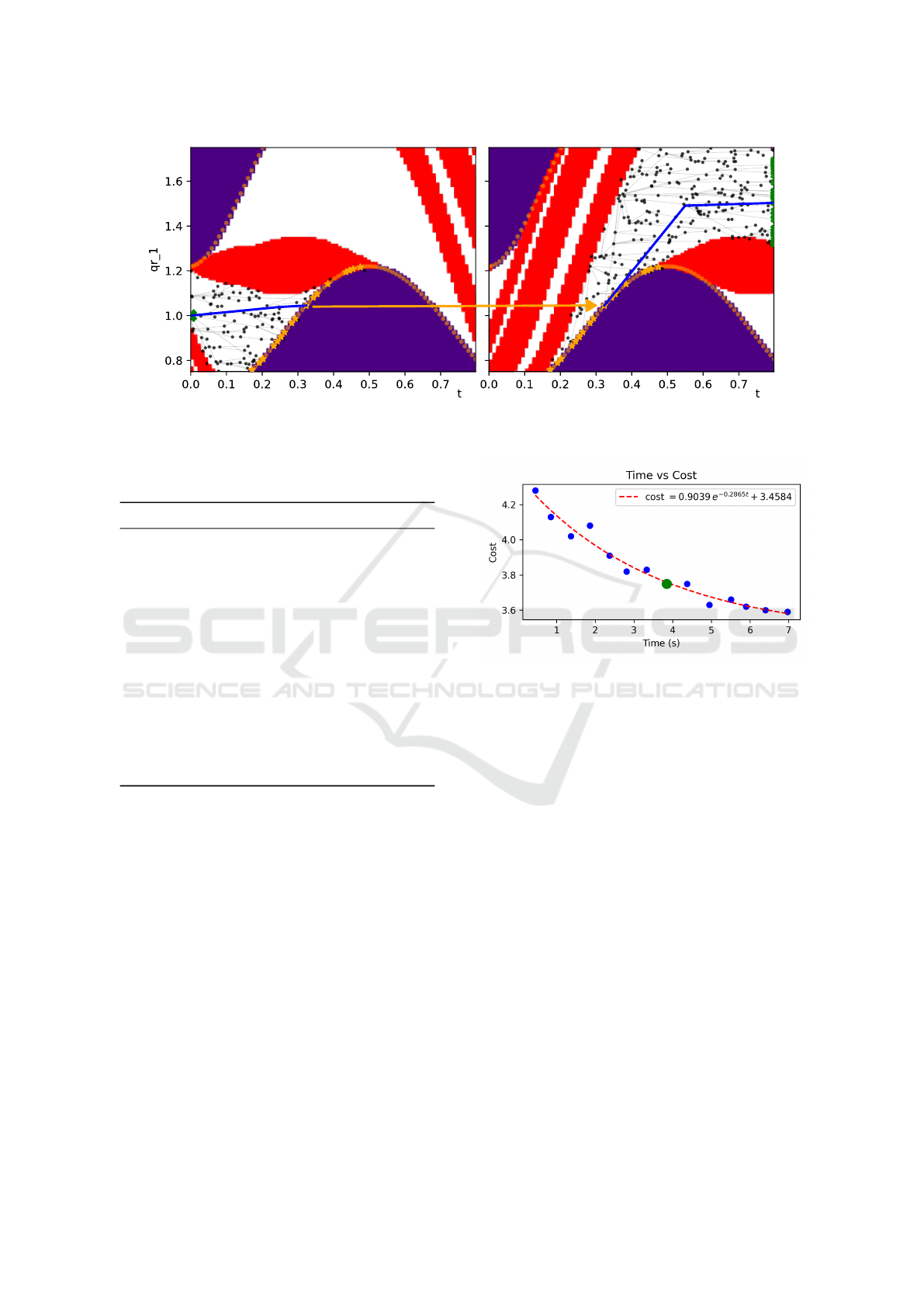
(a)
Transition between FMs
(b)
Figure 4: Feasibility maps and MultiFM-RRT tree for the Stewart platform executing the task trajectory. (a) FM for the first
extended aspect (a = 1). (b) FM for the second extended aspect (a = 2).
Table 2: Performance results of MultiFM-RRT for the
Stewart platform.
i
max
Runtime (s) Cost of P Success rate
250 0.45 4.28 0.76
500 0.85 4.13 0.83
750 1.37 4.02 0.84
1000 1.86 4.08 0.95
1250 2.37 3.91 0.94
1500 2.81 3.82 0.98
1750 3.33 3.83 0.98
2000 3.85 3.75 0.99
2250 4.37 3.75 1.00
2500 4.95 3.63 1.00
2750 5.51 3.66 1.00
3000 5.90 3.62 1.00
3250 6.40 3.60 1.00
3500 6.97 3.59 1.00
counts. The success rate is defined as the propor-
tion of trials in which the algorithm finds a continuous
path that reaches the goal time t
goal
, thereby complet-
ing the prescribed task trajectory.
Figure 5 shows the relationship between runtime
and cost for the different tested values of i
max
. Fitting
a curve to the data reveals a clear exponential trend: as
the cost decreases, runtime increases, and vice versa.
Notably, the trade-off plateaus beyond a certain point,
indicating diminishing returns for further increases in
i
max
. Based on this analysis, we selected i
max
= 2000
as the optimal balance between runtime and solution
quality for this example. This value was used in the
experiment shown in Figures 3 and 4, and its perfor-
mance is highlighted in Table 2.
Figure 5: Relationship between runtime and cost of the so-
lution path for different i
max
values.
5 CONCLUSIONS
This paper presented MultiFM-RRT, a novel algo-
rithm for redundancy resolution in kinematically re-
dundant manipulators based on the exploration of
multiple feasibility maps (FMs). By incorporating
singularity maps into the RRT framework, MultiFM-
RRT efficiently explores the space of feasible solu-
tions, enabling transitions between different aspects
and ensuring comprehensive coverage of the solution
space. The algorithm computes FMs online, avoid-
ing the computational burden of precomputation, and
uses probabilistic sampling to guide exploration to-
ward both goal and singularity sets.
The proposed approach was demonstrated on a
Stewart platform, where MultiFM-RRT successfully
generated feasible, collision-free trajectories that sat-
isfied all task and kinematic constraints. Experimen-
tal results showed that the algorithm achieves high
success rates and quickly converges to high-quality
solutions, even with moderate iteration counts. The
ability to autonomously transition between FMs via
ICINCO 2025 - 22nd International Conference on Informatics in Control, Automation and Robotics
164

SMs proved essential for solving tasks with complex
constraints and multiple aspects.
Future work will focus on extending the algorithm
to more complex robotic systems, incorporating ad-
ditional constraints such as dynamic limits. Experi-
ments with real robots will also be conducted to vali-
date the approach in practical scenarios.
ACKNOWLEDGEMENTS
Work supported by grant PRE2021-099226, funded
by MCIN/AEI/10.13039/501100011033 and the
ESF+, and by project PID2024-159765OA-I00,
funded by the State Research Agency of the Spanish
Government.
REFERENCES
Albu-Sch
¨
affer, A. and Sachtler, A. (2023). Redundancy
resolution at position level. IEEE Transactions on
Robotics.
Borrel, P. and Li
´
egeois, A. (1986). A study of multiple
manipulator inverse kinematic solutions with applica-
tions to trajectory planning and workspace determi-
nation. In Proceedings. 1986 ieee international con-
ference on robotics and automation, volume 3, pages
1180–1185. IEEE.
Burdick, J. W. (1989). On the inverse kinematics of re-
dundant manipulators: Characterization of the self-
motion manifolds. In Advanced Robotics: 1989: Pro-
ceedings of the 4th International Conference on Ad-
vanced Robotics Columbus, Ohio, June 13–15, 1989,
pages 25–34. Springer.
Fabregat-Ja
´
en, M., Peidr
´
o, A., Colombo, M., Rocco, P., and
Reinoso,
´
O. (2025). Topological and spatial analysis
of self-motion manifolds for global redundancy reso-
lution in kinematically redundant robots. Mechanism
and Machine Theory, 210:106020.
Fabregat-Jaen, M., Peidro, A., Gil, A., Valiente, D., and
Reinoso, O. (2023). Exploring feasibility maps for
trajectory planning of redundant manipulators using
rrt. In 2023 IEEE 28th International Conference
on Emerging Technologies and Factory Automation
(ETFA), pages 1–8. IEEE.
Fabregat-Ja
´
en, M., Peidr
´
o, A., Gonz
´
alez-Amor
´
os, E., Flo-
res, M., and Reinoso, O. (2024). Augmented feasi-
bility maps: A simultaneous approach to redundancy
resolution and path planning.
Ferrentino, E. and Chiacchio, P. (2020). On the optimal
resolution of inverse kinematics for redundant manip-
ulators using a topological analysis. Journal of Mech-
anisms and Robotics, 12(3):031002.
Kazemipour, A., Khatib, M., Al Khudir, K., Gaz, C., and
De Luca, A. (2022). Kinematic control of redundant
robots with online handling of variable generalized
hard constraints. IEEE Robotics and Automation Let-
ters, 7(4):9279–9286.
P
´
amanes G, J. A., Wenger, P., and Zapata D, J. L. (2002).
Motion planning of redundant manipulators for spec-
ified trajectory tasks. Advances in Robot Kinematics:
Theory and Applications, pages 203–212.
Peidro, A. and Haug, E. J. (2023). Obstacle avoidance in
operational configuration space kinematic control of
redundant serial manipulators. Machines, 12(1):10.
Peidro, A., Reinoso, O., Gil, A., Mar
´
ın, J. M., and Paya,
L. (2018). A method based on the vanishing of
self-motion manifolds to determine the collision-free
workspace of redundant robots. Mechanism and Ma-
chine Theory, 128:84–109.
Reveles, D., Wenger, P., et al. (2016). Trajectory planning
of kinematically redundant parallel manipulators by
using multiple working modes. Mechanism and Ma-
chine Theory, 98:216–230.
Wenger, P., Chedmail, P., and Reynier, F. (1993). A global
analysis of following trajectories by redundant manip-
ulators in the presence of obstacles. In [1993] Pro-
ceedings IEEE International Conference on Robotics
and Automation, pages 901–906. IEEE.
Whitney, D. E. (1969). Resolved motion rate control of ma-
nipulators and human prostheses. IEEE Transactions
on man-machine systems, 10(2):47–53.
Zanchettin, A. M. and Rocco, P. (2017). Motion planning
for robotic manipulators using robust constrained con-
trol. Control Engineering Practice, 59:127–136.
Redundancy Resolution in Multiple Feasibility Maps via MultiFM-RRT
165