On the Synthesis of Stable Switching Dynamics

to Approximate Limit Cycles of Nonlinear Oscillators

Nils Hanke

, Zonglin Liu

and Olaf Stursberg

Control and System Theory, EECS Dept., University of Kassel, Germany

Keywords:

Oscillators, Limit Cycles, Approximation, Switching Afﬁne Systems, Stability.

Abstract:

This paper presents a novel method for approximating periodic behavior of nonlinear systems by use of switch-

ing afﬁne dynamics. While previous work on approximating limit cycles by switching systems has been re-

stricted t o state space partitions with only two regions or approximations in the plane, this study employs more

general partitions in higher-dimensional spaces as well as external signals to develop a scheme for synthesiz-

ing models with guaranteed existence of a globally stable limit cycle. The synthesis approach is formulated

as a constrained numeric optimization problem, starting from sampled nonlinear dynamics data. I t minimizes

deviations between this data and the switching afﬁne model’s limit cycle, while satisfying constraints to ensure

global stabilit y. The principle and effectiveness of the proposed method is illustrated through examples.

1 INTRODUCTION

Periodic behav ior is a fundamental phenomenon ob-

served across numer ous application do mains, includ-

ing biology, engineer ing, and physics (Teplinsky

and Feely, 2008; Mirollo and Strogatz, 1990; Pe-

terchev and Sanders, 2003). While nonlinear oscilla-

tor models such as Kuramoto, Van-der-Pol, FitzHugh-

Nagumo, Dufﬁng, or Goodwin oscillators (Kuramoto,

2005; Josh i et al., 2016; Gaiko, 2011; D¨orﬂer and

Bullo, 2014; Kudry ashov, 2021; Gonze and Ruoff,

2021; Atherto n and Dorrah, 19 80) ar e widely u sed

to d e scribe periodic behavior, the an a lysis of these

models is limited: Speciﬁcally, the characteriz ation

and ana lysis of limit cycles, including conditions for

uniqueness and stability, is often restricted to special

cases. A central challenge in studying such behavior

is to approximate the underlying oscillatory dynam-

ics with an analytically tractable system class which

allows to rigorously analyze its properties. Exist-

ing data-driven approach es, such as machine learn-

ing or hybrid system identiﬁcation, can approximate

periodic behavior (X u and Luo, 2019), but they are

not designe d to allow for rigorous analysis of proper-

ties of limit cycles. This gap hinde rs the systematic

study of oscillatory phenomena in applications such

as, e.g., the investigation of circadian rhythms in bio-

logical systems (Werckenth in et al., 2020), where un-

https://orcid.org/0009-0008-8940-2677

https://orcid.org/0000-0002-0196-9476

https://orcid.org/0000-0002-9600-457X

derstandin g stability, phase shifts, and synchroniza-

tion is essential.

To simplify the model analysis, switching or

piecewise-afﬁne systems (PAS) have proven effective

in appr oximating nonlin e ar dy namics (Paoletti et al.,

2007; Lauer et al., 2011). This is primarily due to

the facts that (1.) the analytic solution of piecewise-

afﬁne systems exists for each region of the parti-

tioned state space, and (2.) the approximation qual-

ity can be tuned through adapting the partitioning and

parametriza tion. Speciﬁcally with respect to the ap-

proxim ation of nonlinear systems with periodic tra-

jectories, the work in (Lum and Chua, 1991; Freire

et al., 1998) proposed conditions f or the existence of

limit cycles of PAS (with two-r egio n partitions) in R

The uniquene ss and stability of these limit cycles are

further examined in (Coll et al., 200 1; Llibre et al.,

2008). These results are then adopted in (Kai and Ma-

suda, 2012) to synthesize PAS with stable limit cycles

in R

, while the work in (Hanke and Stursb e rg, 2023;

Hanke e t al., 2024) further developed algorithms to

generate p la nar switching afﬁne systems to approxi-

mate given limit cycles with guara ntees of uniqueness

and local stability. However, there the use of only two

afﬁne dynamics and a single separating line limits the

approximation quality. A comprehensive review of

the conditions of the existence of limit cycles in pla-

nar piecewise-linear systems can be found in (Freire

et al., 1998) or in Chapter 5.1 of (Bernardo et al.,

2008). The recent work (Hanke et al., 2025) improved

the approximation quality by employing multiple par-

titions, however the proposed result is still lim ited to

Hanke, N., Liu, Z. and Stursberg, O.

On the Synthesis of Stable Switching Dynamics to Approximate Limit Cycles of Nonlinear Oscillators.

DOI: 10.5220/0013835000003982

Paper published under CC license (CC BY-NC-ND 4.0)

In Proceedings of the 22nd International Conference on Informatics in Control, Automation and Robotics (ICINCO 2025) - Volume 1, pages 509-516

ISBN: 978-989-758-770-2; ISSN: 2184-2809

509

the R

, and it lacks the guarantee o f global stability

of the limit cycle.

This paper extends the approaches in literature to

higher-dimensional spaces by leveraging the contrac-

tion p roperty outlined in (Pavlov et al., 2007) to gen-

erate PAS with globally stable limit cycles. A novel

method is proposed for partitioning the state space

and sy nthesizing afﬁne dynam ics within each region,

ensuring both global stability and adjustable approxi-

mation quality.

Section 2 ﬁrst introduces properties of PAS which

are essential for ensuring high approximation quality.

Section 3 proposes rules for partitioning state spaces

of arbitrary dimensions and for synthesizing PAS with

desired p roperties by use of optimiza tion. An illustra-

tive numerical example is presented in Sec. 4, includ-

ing cases in 2 and 3 dimen sio ns, before conclusions

and an outlook are provided in Sec. 5.

2 PROBLEM DESCRIPTION

The objective of the procedure to be proposed in this

paper is to reconstruct limit cycles of a broad class of

oscillatory systems with the following property: T he

underlying nonlinear dynamics (deﬁned in R

) gen-

erates a smo oth and stab le limit cycle which 1.) is

embedd ed in an (n

− 1)-dim. manifold, 2.) oscillates

around a virtual center point, and 3.) does not show

strong twisting nor points of intersection with itself.

Assume that an or dered set F := { ˜x

, ˜x

, .. . , ˜x

}

of different state samples ˜x

∈ R

is taken along

the limit cycle of the n onlinear dynamics. For the

sake of clarity, it is assumed that the sampling time

∆t is constant along the cycle, while the method in-

troduced later is also applicable to cases with non-

unifor m sampling times. The sampling is assumed to

be dense in the sense that n

is much larger than n

i.e., the sampling time ∆t is much smaller than the pe-

riod T = n

·∆t of the limit cycle, and ∆t < 1 applies.

Given F, the o bjective of this paper is to propose

a method to construct a dynamic model approximat-

ing the limit cycle of the non linear dynamics wh ile

preserving its properties – for this purpose, the class

of switching afﬁne systems is chosen: Let x(t) ∈ R

denote the state at time t ∈ R and u(t) ∈ R a scalar in-

put signal, which is multiplied by a vector B ∈ R

×1

Assume th at the state space R

is partitioned into

ﬁnitely many polytop es P

⊆ R

, i ∈ {1, . . . , n

which are parametrized by C

∈ R

1×n

, d

∈ R, and

= C

, d

= d

accordin g to:

:={x∈R

x≥d

i+1

x<d

i+1

[

i=1

. (1)

Note that this deﬁnition is particular in the sen se that

the number of P

and bound ing planes (C

, d

) is both

, as required for the procedure to be proposed. For

pairs (A

, b

) of A

∈ R

×n

and b

∈ R

×1

, the afﬁne

dynamics assigned to each P

is:

˙x(t) = A

x(t) + b

+ Bu(t), for x(t) ∈ P

. (2)

Consider a set of switching tim e s T

= {t

, . . .} with

the initial time t

= 0. A trajectory ¯x

[0,∞[

of (2), start-

ing from the initial state x(t

) = x

, contains the state

evolution for a sequence of phases [t

k+1

] in between

two successive switching times. In each phase with

t ∈ [t

k+1

], the pair (A

, b

) in (2) is activated for the

index i for which x(t) ∈ P

applies. A limit cycle, as a

particular trajectory of (2), is deﬁned a s follows:

Deﬁnition 1. Limit Cycle

A trajectory ¯x

∗

[0,∞[

of (2) is called limit cycle, if a ﬁnite

period T ∈ R

exists such that for any po int x(t) ∈

¯x

∗

[0,∞[

, t ∈ R

≥0

it applies that: x(t + T) = x(t). 

Deﬁnition 2. Stability of a Limit Cycle

A limit cycle ¯x

∗

[0,∞[

of (2 ) is called globally stable, if

every trajectory converges to wa rds ¯x

∗

[0,∞[

indepen dent

of the initialization x(0) = x

∈ R

. 

The identiﬁcation of a model of type (2) from F

requires to synthesize the following parameters: 1.)

the number n

of elements P

of the state space parti-

tion, 2.) the boundar ies C

x = d

of the P

, 3.) the pair

of matrices (A

, b

) for each P

, and 4.) the signal u(t)

together with the vector B. To match the p roperties

assumed for the limit cycle of the nonlinear system,

the particular synthesis requireme nts are:

• The evolution of (2) also forms a limit cycle ¯x

∗

[0,∞[

which is globally stable according to Def. 2.

• The period of the limit cycle ¯x

∗

[0,∞[

is T = n

· ∆t.

• The limit cycle ¯x

∗

[0,∞[

tracks the sample points in

F as well as p ossible.

Switching afﬁne systems are a promising candid a te

for such an approximation, since the number of pa-

rameters in each P

is small and th e dynamics is rela-

tively simple to analyze. In particular, if the con sid -

ered dynamics is strongly nonlinear along the cycle,

the approximation with afﬁne dynam ic s in restricted

regions is well justiﬁed, while freedom in choosing

the P

(wrt. number and positioning) allows in princi-

ple to obtain arbitr a rily good approximations. How-

ever, most existing work on approximating limit cy-

cles is limited to either two regions in the plane, o r

provides only local stability guarantees. To address

these limitations, the following exposition uses the

concept of contractivity to obtain a synthesis proce-

dure achieving the named properties of ¯x

∗

[0,∞[

by nu-

merical optimization.

ICINCO 2025 - 22nd International Conference on Informatics in Control, Automation and Robotics

510

3 SYNTHESIS OF CONTRACTIVE

SWITCHING AFFINE SYSTEMS

3.1 Partitioning of the State Space

In order to fully utilize the degrees of freedom of-

fered by (2) in assigning different afﬁne dynamics to

the r egions when tracking the set of samples F :=

{ ˜x

, ˜x

, . . . , ˜x

}, a method for partitio ning the state

space in any dimension n

∈ [2, n

− 1] is introduced

ﬁrst. This method ensu res that the resulting partition

satisﬁes the conditions in (1). Speciﬁcally, the cases

of n

= 2, n

= 3, and n

> 3 are discussed separately

in the sequel.

Case n

= 2

: Let a cen te r point x

of all points in

F be determined by:

s,[q]



max

l∈{1,...,n

}

˜x

l,[q]

− min

l∈{1,...,n

}

˜x

l,[q]



(3)

for both dimensions q ∈ {1, 2}. By assuming that x

does not coincide with any point in F, a set of n

sample points ˆx

, . . . , ˆx

is selected from F, see Re-

mark 2 at the end of this subsection for more details.

Then, for e a ch point ˆx

, a unique line C

x = d

with

∈ R

1×2

, d

∈ R, can be determined, which contains

and ˆx

. Such a lin e then serves as the boundary be-

tween the regions P

i−1

and P

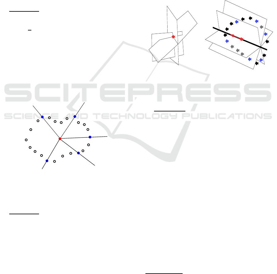
, as illustrated in Fig. 1.

ˆx

Figure 1: Based on F, the center point x

, and a set of se-

lected points ˆx

, . . . , ˆx

∈ F (each representing the ﬁrst state

of any subset F

, . . . , F

along the limit cycle), the lines for

partitioning X into regions P

are determined.

Case n

= 3

: Let the center point x

again be de-

termined by (3). Then, a pla ne Ω

∗

x = ε

∗

with Ω

∗

∈

1×3

, ε

∗

∈ R, is determined by:

(Ω

∗

, ε

∗

) := a rg min

Ω,ε

∑

i=1

kΩ ˜x

− εk

, s.t. Ωx

= ε (4)

Based on the outcome of (4), a line:

Γ := {x ∈ R

| x = x

+ ηΩ

∗

, η ∈ R} (5)

which contains x

and shares the direction vector Ω

∗

is obtained. Note that the plane Ω

∗

x = ε

∗

contains the

center point x

, while the overall distance between the

sample p oints in F to the plane is minimized across

all possible values of Ω and ε. If no point in F is

contained

in Γ, a set of n

sample points ˆx

, . . . , ˆx

is selected from F. For each of these sam ple points

ˆx

, a unique plane containing ˆx

and the line Γ is de-

termined. If su ch a plane does not contain any other

sample p oint fr om F, th en it is assumed to constitute

the boundar y R

i−1,i

:= {x ∈ R

x = d

} between two

adjacent regions P

i−1

and P

. In this way, a partition

which does not satisfy (1), as illu strated in Fig. 2a), is

avoided. An admissible partitioning from the afore-

mentioned procedure is shown in Fig. 2b).

Ω

∗

ˆx

Figure 2: For n

= 3, the partitioning shown i n Fig. 2 a)

does not satisfy (1). In contrast, an admissible partition is

obtained by the considered procedure for the case i n Fi g. 2

b).

Case n

> 3:

Determine aga in x

, the vector Ω

∗

∈

1×n

, and the line Γ accor ding to ( 3) to (5). Let also

sample p oints ˆx

, . . . , ˆx

be selected fr om F. How-

ever, for any of these sample points ˆx

, a hyperplane

containing ˆx

and the line Γ (while being deﬁned in

an n

− 1 dimensiona l subspace) is not unique. To re-

solve this issue, a set of linearly independent vectors

Ω

, . . . , Ω

−2

, Ω

∈ R

1×n

, ar e ide ntiﬁed, which have

to be linea rly independent of Ω

∗

. Based on these vec-

tors, a hyperplane Ψ can be determined in the n

− 2

dimensional subsp a ce by:

Ψ:={x ∈ R

|x = x

+η

Ω

∗

−2

∑

j=2

Ω

, η

∈ R}. (6)

Assume that Ψ does not contain any points from F,

then for ea ch sample point ˆx

, a unique hyperplane in

the n

− 1 d imensional subsp ace can be determined,

which contains Ψ and ˆx

. If such hyperplane does not

contain any o ther sample point from F , this hyper-

plane is then chosen to be the boundary R

i−1,i

:= {x ∈

x = d

} between the regions P

i−1

and P

Remark 1 . The proposed procedure a-priori ex-

cludes sets F that are likely to yield poor approxi-

If this condition does not hold, one may resolve the

issue by slightly changing Ω

∗

On the Synthesis of Stable Switching Dynamics to Approximate Limit Cycles of Nonlinear Oscillators

511

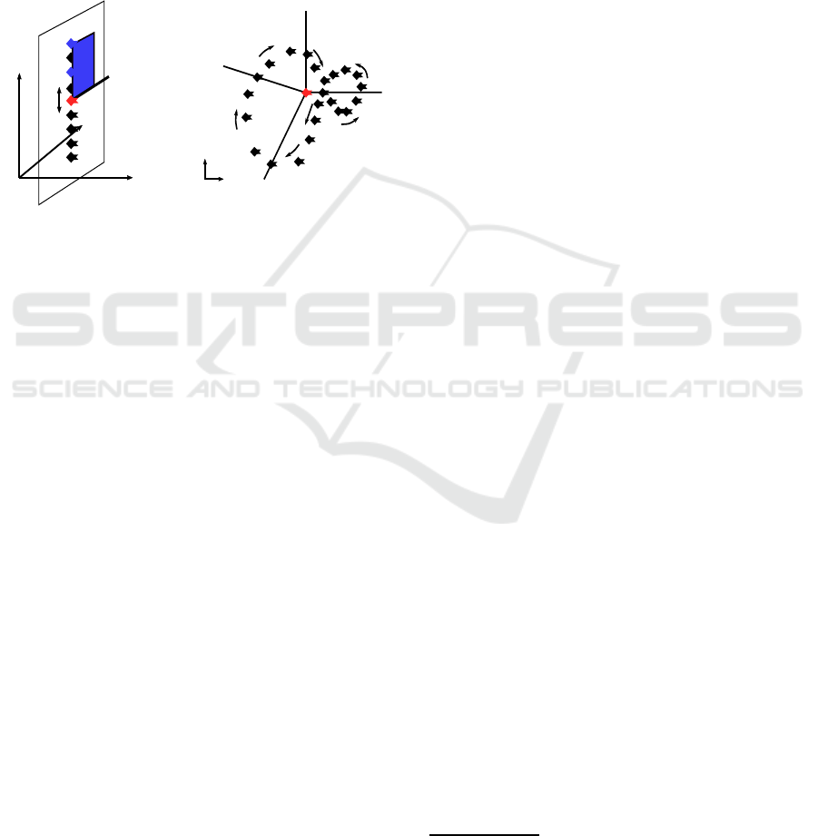
mations. One of these c ases is sho wn in Fig. 3 a),

in which the condition is not satisﬁed that C

x = d

does only contain one sample point ˆx

and one lin e Γ.

The second case, shown in Fig. 3 b), correspon ds to

a limit cycle intersecting itself. While the proposed

partitioning procedure may succeed here, it becomes

clearly evident, e.g. for P

, that no afﬁne system can

be found that adequately captures the opposing d irec-

tions of motion of the trajectories. This limitation mo-

tivates the exclusion of limit cycles with intersections,

as stated in Sec. 2.

ˆx

Ω

∗

x = ε

∗

x = d

Figure 3: Types of sets F that are not suitable for the par-

titioning procedure under consideration: the case in a) fails

to meet the condition that C

x = d

does only contain a sam-

ple point ˆx

and Γ, while the case in b) is not feasible for

determination of A

, b

∈ P

and A

, b

∈ P

Remark 2. The n

sample points of the sequence

{ ˆx

}

i=1

with timestamps {

}

i=1

are selected from F

such that all time intervals satisfy:

∆

:= |

i+1

−

| < 1 ∀i ∈ {1, . . . , n

} (7)

with

≡ t

. While this selec tion is not strictly nec-

essary to partition the state space, it ena bles good ap-

proximation quality in the reconstructed limit cycle,

as will be discussed in Sec. 3.3.

3.2 Construction of the Dynamics

Assume that the number n

and the partition (1 ) into

are ﬁxed. Accord ing to (Pavlov et al., 2007), the

switching afﬁne system (2) is said to be contractive,

if the following is satisﬁed:

• Conditio n 1: A

x + b

= A

i+1

x + b

i+1

holds for

all x on the boundary C

x = d

and for all i ∈

{1, . . . , n

}, with A

= A

and b

= b

• Conditio n 2: A

Q + QA

≺ 0 holds for all i ∈

{1, . . . , n

} with a positive-deﬁnite matrix Q ≻ 0.

The ﬁrst condition requ ires that the gradient of the

autonomous dynamic s on the switchin g b oundaries

must be continuous, while the second condition im-

plies the existence of a common Ly apunov function

in all regions. N ext, the important property of con-

tractivity is established, which underlies the sy nthesis

proced ure in this paper:

Lemma 1. (Contractive switching afﬁne systems

(Demidovich, 1967; Pavlov et al., 2007)) I f the sys-

tem (2) is contractive with a non-zero vector B, then

for any piecewise continuous periodic signal u(t) with

a period T , the solution x(t), t ≥ 0 starting from an ar-

bitrary x(0 ) ∈ R

always converges to a unique limit

cycle with the same period T . 

In order to enco de the requirement of continu-

ous gradients on the switchin g boundaries, the fol-

lowing equality constraints for syn thesizing (A

, b

i ∈ {1, . . . , n

} are proposed:

i,[q]

−A

i+1,[q]

=α

i,[q]

, b

i,[q]

−b

i+1,[q]

=α

i,[q]

(8)

for α

i,[q]

∈ R and q ∈ {1, . . . , n

}, where A

i,[q]

repre-

sents the q-th r ow of A

The condition for the existence of a common Lya-

punov function represents a nonlinear matrix in e qual-

ity involving the matrices A

, . . . , A

and Q. If these

constraints are satisﬁed, th e system (2) is ensured to

have a globally stable limit cycle as in Def. s 1 and

2 with a period of T (provided that the signal u(t)

is also periodic with the same length, see Lemma 1).

The task is thus to adapt ( 2) in order to a chieve that

the limit cycle approximates the sample points in F

with respect to position and time.

3.3 Tracking the Sample Points in F

For tracking the sample points in a set F

, consider the

set F

explicitly – the following procedure can then be

transferred to the other sets F

, i ∈ {2, . . . , n

} equiva-

lently. For F

= { ˆx

, ˜x

, . . . , ˜x

} with n

denoting the

number of points in F

and ˆx

= ˜x

, the following cost

functional is deﬁned:

∑

j=2

||e

( j−1)∆t

ˆx

+ . . .

( j−1)∆t

(( j−1)∆t−τ)

+ Bu(τ)) dτ − ˜x

. (9)

It records the difference betwe en the rea c hable points

of ˙x(t) = A

x(t) + b

+ Bu(t) (starting from ˆx

) and

the sampled points in F

at each sampling time

By synthesizing A

, b

and B for a given signal

u(t), the ﬁrst challenge in minimizing J

is the nonlin-

earity caused by the matrix exponential function e

For sampled states in F with non-uniform but known

sampling times, only the corresponding times in (9) need to

be adjusted.

ICINCO 2025 - 22nd International Conference on Informatics in Control, Automation and Robotics

512

Based on the Taylor series:

+. . .≈I

∑

j=1

(10)

the value of e

can be approximated by the right-

hand side of (10) with sufﬁciently high order n

. If

the state dimension n

is large, a high order n

would

increase the complexity of the optimization signiﬁ-

cantly (due to a higher-order non linearity), whereas

a smaller order (such as n

≤ 3) would lead to a non-

negligible approximation error. To this end, two pos-

sible countermeasures are introduced:

• For a ﬁxed matrix A

, the approximation error in

(9) is small for small times t. Especially for t < 1

the series t

, j ∈ {n

, n

+ 1 , . . .} in th e neglected

terms is converging to zero, and thus neglecting

these terms does only lead to small contributions

to the approximation error.

• For any ﬁxed time t and if the spectru m of A

is contained in the unit cycle, the matrices A

j ∈ {n

, n

+ 1, . . .} in the neglected terms also

conve rge to zero, thus leading to small errors.

The ﬁrst countermeasure is included into the parti-

tioning procedure in Section 3.1 Remark 2 by se-

lecting sam ple points on the boundar ie s such that

j · ∆t < 1 holds for all j ∈ {1, . . . , n

} in (9). The sec-

ond countermea sure is established by e nsuring that

the largest sing ular value of A

is smaller than one ,

what can be guaranteed by ob serving the nonlinear

matrix inequality:

≺ I

. (11)

Note that larger numbers n

of regions of the parti-

tion, in general, reduce the tr a nsition time from one

boundary to the next, and thus lead to smaller ap-

proxim ation errors in the Taylor series expan sion fo r

a given order n

(at the price of having to synthesize

more p a irs (A

, b

)). The condition (11) forces the

eigenvalues of A

to be contained in the interior of the

left half of the unit circle (since the contraction co n-

dition requires the real-part o f the eige nvalues of A

to be negative in add ition). Consequently, the conver-

gence rate of (2) in the region P

is also bounded by 1,

which can be cou nterproductive if the samp le points

to be tracked in F

encode that the state of the sampled

limit cycle changes very differently in a certain region

of th e state space. As a re sult, the inclusion of (11 )

should be seen as an o ptional me a sure, or be replaced

by a less conservative condition, such as A

≺ βI

for some β > 1. The described countermeasures only

affect the approximation quality withou t compr omis-

ing th e contraction property ensured by Lemma 1. A

detailed a nalysis of the upper bound of the approxi-

mation error can be found in (Higham, 2009; Kenney

and Laub, 1998).

The periodic signal u(t) can e.g. be chosen piece-

wise constant for k ∈ {0, 1, 2, . . .}:

u(t) =

(

−1, t < [kT, (k +

)T )

1, t < [(k +

)T,(k + 1)T ).

(12)

The integral part of (9) then le a ds to an analytic ex-

pression:

(t−τ)

+ Bu(τ)) dτ =











− I

−1

− B) for 0 ≤ t <

−I

−1

−B)+(e

(t−

T )

−I

−1

+B)

for

T ≤ t < T,

what is particularly beneﬁcial for applying the pre-

viously discussed countermeasures in synthesis, see

Section 3.4. Note that the matrix A

is always in-

vertible, as the contractivity condition implies that A

must be Hurwitz.

3.4 Overall Optimization Problem

Given a partitioned state space according to Sec. 3.1

and a periodic signal u(t) of type (12), the optimiza-

tion problem to synthesize the switching afﬁne system

(2) is deﬁned as:

min

,α

,i∈{1,...,n

},B,Q

∑

i=1

(13)

s.t. for all i ∈ {1, . . . , n

} :

constraints (8) ∀q ∈ {1, . . . , n

}, (14)

Q + QA

≺ 0, Q ≻ 0, B 6= 0, (15)

≺ I

(option al constraint), (16)

∆t

ˆx

∆t

∆t−τ)

+Bu(τ))dτ= ˆx

i+1

. (17 )

In h ere, J

is deﬁned fo r each region in a sim ilar way

as J

in (9). This is a nonlinear optimization problem

with in total (n

+ 1 )n

+ (2n

+ 1 )n

variables. The

cost func tional minimized in (13) r ecords the distance

between each sample point in F and the point on the

limit cycle of (2) at the same time. The c onstraints

(14) and (15) guarantee that the resulting sy stem (2)

is contrac tive, while the optio nal constraint (16) aims

at achieving a satisfying approximation by using the

Taylor expansion f or the matrix exponential function

in (13) and (17). The last constraint aims at ensur-

ing that the set of sam ple points ˆx

, i ∈ {1, . . . , n

}

on the boundaries are reached by the limit cycle of

(2). Otherwise, the minimization of (13) may only

On the Synthesis of Stable Switching Dynamics to Approximate Limit Cycles of Nonlinear Oscillators

513

force a transient trajectory of (2) to track the sample

points in F, instead of the limit cycle of (2 ) (due to

the appro ximation error of e

). In general, the op-

timization problem is not guaranteed to be feasib le ,

but increasing the number n

or choosing a d ifferent

partition contributes to ﬁnding a feasible solution.

As an extensio n to account for transient behavior

from arbitrary initial states to the limit cycle, an ad-

ditional term can be included in (13) to minimize the

deviation of the model dynamics from the sampled

transient trajectories. Finally, it is worth mentioning

that measurem e nt noise ( typically affecting the sam-

ples in F) is eliminated by the solution of (13) to (17)

and assigning the model (2) to any of the regions P

4 NUMERIC EXAMPLES

4.1 Illustrating Example in the Plane

To evaluate the performance of the proposed synthe-

sis method, ﬁrst an example of a set F of nineteen

points in the plane is c onsidered, as shown in Fig. 4

and Fig. 5 (marked by the solid black circles). The

obtained period based on the sample set is T = 1.4,

which is also used f or the periodic signal (12). In a

ﬁrst instance, the state space is partitioned by eight

rays (solid blue lines) according to the rules provided

in Section 3 with:



1 −



, C



1 −2



, C



−1 −2





−1 −



, C



−1



, C



−1 3







, C





, d

= −3,

=−5, d

=−

, d

=−

, d

=5, d

=6, d

using the center point x

= [1, 2]

. The limit cycle of

(2) obtained from solving the proble m (13) with an

order of n

= 4 for the ma trix exponential function is

shown in Fig. 4. The shape of the limit cycle makes

apparent that a small order n

leads to considerable

approximation errors. As a countermeasure, the order

is increased to n

= 9, for which the pairs (A

, b

i ∈ {1, . . . , 8} are obtained from solving the problem

(13) (again with T = 1.4 in (12)). The resulting limit

cycle is marked in black in Fig. 5.

The distance to the sampled points is much

smaller, and trajectories from different initial p oints

(in- and outside of the limit cycle) are simulated to

demonstra te the stability and uniqueness of the limit

cycle, see Fig. 5 and Fig. 6 (so lid mage nta, red and

green). Note that the optional condition (1 6) was not

used within this optimization, since the accuracy of

the matrix exponential with n

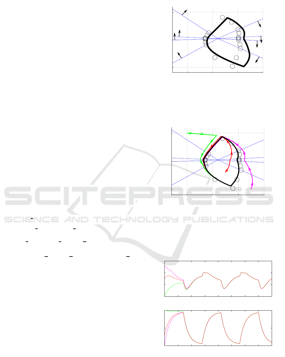
= 9 was acceptable.

−50

−5

Figure 4: Sample points (black circles), switching bound-

aries in solid blue, and the limit cycle of the switching sys-

tem with n

= 4 in solid black.

−50

−5

, b

Figure 5: Sampled points (black circles) and switching

boundaries in blue. The limit cycle is shown in black as well

as trajectories from different initial points x(0)=



2.5 −20



red, x(0)=



−5 50



green, and x(0)=



7.5 −50



magenta.

0 0.5 1 1.5 2 2.5 3 3.5 4

-5

(t)

0 0.5 1 1.5 2 2.5 3 3.5 4

-50

(t)

Figure 6: Convergence of x

(t) and x

(t) for different initial

points x(0)=



2.5 −20



red, x(0)=



−5 50



green, and

x(0)=



7.5 −50



magenta.

ICINCO 2025 - 22nd International Conference on Informatics in Control, Automation and Robotics

514

4.2 Example i n a 3D-Space

For an add itional example w ithin a 3-dimensiona l

state space, consider the set of sample points illus-

trated in Fig. 7 (denoted by blac k circles). By apply-

ing the method described in Section 3.1 ( case n

= 3),

and adhering to the requirement of the ﬁrst counter-

measure (transition times between sam ple points on

adjacent boundaries are less than 1 ) leads to n

= 8

subsets F

to minimize the transition time between

each pair of ˆx

. Solving the optimization pro blem (4)

and using the provided sample points as well as the

center point x

= [1, 2, 0]

provides the following re-

sult:

Ω

∗



−0.0115 −0.0066 0.9999



, ε

∗

= −0.0247,

which is shown as green plane in Fig. 7. The required

line of intersectio n is give n by Γ := {x ∈ R

| x =

+ ηΩ

∗

, η ∈ R}, as marked by the solid blue line

in Fig. 7. Since no point in F is contained in Γ, a

unique plane containing both ( Γ and ˆx

) is determined

for each sample point ˆx

to:



1 −

0.0099



, C



1 −2 −0.0017





−1 −2 −0.0247





−1 −

−0.0132





−1

−0.0102



, C



−1 3 0 .0083





0.0280



, C



0.0126



, d

=0.5, d

=−3

=−5, d

=−1.5, d

=−0.6, d

=5, d

=6, d

=1.33,

see the solid blue planes in Fig. 7. The resulting limit

cycle o btained from solving the optimization problem

in Sectio n 3.4 is marked in black in Fig. 7. The dis-

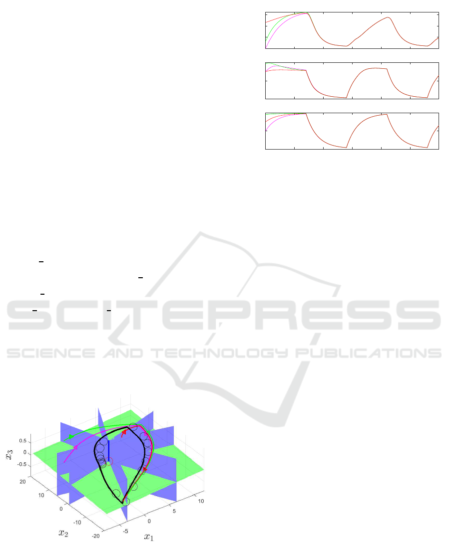
tance to the sampling points is onc e again acceptable,

Figure 7: Sampled points (black circles), green plane with

minimum distance to the sampled points i ncluding x

(red

circle), the line of intersection Γ as solid blue line and

boundaries shown as planes in blue, while the limit cycle

is marked in black and the trajectories from different initial

points x(0)=



6.5 10 0.1



red, x(0)=



−1.9 18.5 0.18



green, and x(0)=



−5 10 0



magenta.

0 0.5 1 1.5 2 2.5 3

-5

(t)

0 0.5 1 1.5 2 2.5 3

-20

(t)

0 0.5 1 1.5 2 2.5 3

-0.2

0.2

(t)

Figure 8: Convergence of x

(t), x

(t) for dif-

ferent initial points x(0) =



6.5 10 0.1



red, x(0) =



−1.9 18.5 0.18



green, and x(0)=



−5 10 0



magenta.

even though a ll dimensions are on signiﬁcantly dif-

ferent scales, which underscores the approximation

quality of the approach. Trajectories from different

initial points again demonstrate the convergence to

the unique limit cycle, see Fig. 7 an d Fig. 8 with tra-

jectories in magenta, red, and green.

5 CONCLUSIONS

This work has introduced a method for approximat-

ing periodic behavior of non linear dynamic systems

not restricted to the planar case. Based on suitable

sampling of the limit cycle of th e nonlinear dynam-

ics, switched afﬁne systems with exogenous inputs

are used for app roximation, wh ile the approach pre-

serves essential limit cycle properties including stabil-

ity and u niqueness. Unlike previously available meth-

ods, the work here provides constructive rules to par-

tition the state space and synthesize the dynam ic s by

optimization, such that the limit cycle of the switching

afﬁne system matches the sample points of the non-

linear data generator in an optimized sense. By using

the notion of contractivity, the constructed limit cycle

is ensured to be globally stable. Although the intro-

duced conditions generate a non-convex and nonlin-

ear optimization problem, they simultaneously ensure

a smooth limit cycle, a behavior freq uently observed

in real-world systems. While solvability of the opti-

mization pr oblem cannot be guaranteed, any solution

found under these conditions will be convergent.

It should be noted that the use of a center point in

which all boundaries intersect is p articularly suitable

if the sample points have a relatively even distribution

around an interior region in R

On the Synthesis of Stable Switching Dynamics to Approximate Limit Cycles of Nonlinear Oscillators

515

Future work aims at investigating schemes of par-

titioning without a common center point, and the cou-

pling of severa l oscillators of the proposed type.

ACKNOWLEDGEMENTS

Partial ﬁnancial support by the G e rman Research

Foundation (DFG) through the Research Training

Group Biological Clocks on Multiple Time Scales

(GRK 2749/1) is gratefully acknowledged.

REFERENCES

Atherton, D. and Dorrah, H. (1980). A survey on non-

linear oscillations. International Journal of Control,

31(6):1041–1105.

Bernardo, M., Budd, C., Champneys, A. R., and Kowal-

czyk, P. (2008). Piecewise-smooth dynamical sys-

tems: theory and applications, volume 163. Springer

Science & Business Media.

Coll, B., Gasull, A., and Prohens, R. (2001). Degener-

ate hopf bifurcations in discontinuous planar systems.

Journal of mathematical analysis and applications,

253(2):671–690.

Demidovich, B. P. (1967). Lectures on stability theory.

D¨orﬂer, F. and Bullo, F. (2014). Synchronization in com-

plex networks of phase oscillators: A survey. Auto-

matica, pages 1539–1564.

Freire, E., Ponce, E., Rodrigo, F., and Torres, F. (1998). Bi-

furcation sets of continuous piecewi se linear systems

with two zones. International Journal of Bifurcation

and Chaos, 8(11):2073–2097.

Gaiko, V. A . (2011). Multiple limit cycle bifurcations of the

ﬁtzhugh–nagumo neuronal model. Nonlinear Analy-

sis: Theory, Methods & Applications, 74(18):7532–

7542.

Gonze, D. and Ruoff, P. (2021). The goodwin oscillator and

its legacy. Acta Biotheoretica, 69(4):857–874.

Hanke, N., Liu, Z., and Stursberg, O. (2024). Approxima-

tion of limit cycles by using planar switching afﬁne

systems with guarantees for uniqueness and stability.

In European Control Conference, pages 1460–1465.

Hanke, N., Liu, Z., and Stursberg, O. (2025). Approxima-

tion of planar periodic behavior from data with sta-

bility guarantees using switching afﬁne systems. In

American Control Conference, pages 1944–1949.

Hanke, N. and Stursberg, O. (2023). On the design of limit

cycles of planar switching afﬁne systems. In European

Control Conference, pages 2251–2256.

Higham, N. J. (2009). The scaling and squaring method

for the matrix exponential revisited. SIAM review,

51(4):747–764.

Joshi, S. K., Sen, S., and Kar, I. N . (2016). Synchronization

of coupled oscillator dynamics. I FAC-PapersOnLine,

49(1):320–325.

Kai, T. and Masuda, R. (2012). Limit cycle synthesis of

multi-modal and 2-dimensional piecewise afﬁne sys-

tems. Mathematical and Computer Modelling, 55(3-

4):505–516.

Kenney, C. S. and Laub, A. J. (1998). A schur–fr´echet al-

gorithm for computing the logarithm and exponential

of a matrix. SIAM journal on matrix analysis and ap-

plications, 19(3):640–663.

Kudryashov, N. A. (2021). The generalized dufﬁng oscil-

lator. Communications in Nonlinear Science and Nu-

merical Simulation, 93:105526.

Kuramoto, Y. (2005). Self-entrainment of a population

of coupled non-linear oscillators. In International

symposium on mathematical problems in theoreti-

cal physics. Kyoto University, Japan, pages 420–422.

Springer.

Lauer, F., Bloch, G., and Vidal, R. (2011). A continuous op-

timization framework for hybrid system identiﬁcation.

Automatica, 47(3):608–613.

Llibre, J., Ponce, E., and Torres, F. (2008). On the exis-

tence and uniqueness of limit cycles in li´enard differ-

ential equations allowing discontinuities. Nonlinear-

ity, 21(9):2121.

Lum, R. and Chua, L. O. (1991). Global properties of con-

tinuous piecewise linear vector ﬁelds. part i: Simplest

case in R

. International journal of circuit theory and

applications, 19(3):251–307.

Mirollo, R. E. and Strogatz, S. H. (1990). Synchronization

of pulse-coupled biological oscillators. SIAM Journal

on Applied Mathematics, 50(6):1645–1662.

Paoletti, S., Juloski, A. L., Ferrari-Trecate, G., and Vidal,

R. (2007). Identiﬁcation of hybrid systems a tutorial.

European journal of control, 13(2-3):242–260.

Pavlov, A., Pogromsky, A., Van De Wouw, N., and Nijmei-

jer, H. (2007). On convergence properties of piece-

wise afﬁne systems. International Journal of Control,

80(8):1233–1247.

Peterchev, A. V. and Sanders, S. R. (2003). Quantiza-

tion resolution and limit cycling in digitally controlled

pwm converters. IEEE Transactions on Power Elec-

tronics, 18(1):301–308.

Teplinsky, A. and Feely, O. (2008). Limi t cycles in a mems

oscillator. IEEE Transactions on Circuits and Systems

II: Express Briefs, 55(9):882–886.

Werckenthin, A., Huber, J., Arnold, T., Koziarek, S., Plath,

M. J., Plath, J. A., Stursberg, O., Herzel, H., and

Stengl, M. (2020). Neither per, nor tim1, nor cry2

alone are essential components of the molecular circa-

dian clockwork in the madeira cockroach. PLoS One,

15(8):e0235930.

Xu, Y. and Luo, A. C. (2019). Fr equency-amplitude char-

acteristics of periodic motions in a periodically forced

van der pol oscillator. The European Physical Journal

Special Topics, 228(9):1839–1854.

ICINCO 2025 - 22nd International Conference on Informatics in Control, Automation and Robotics

516