Augmenting Neural Networks-Based Model Approximators in Robotic
Force-Tracking Tasks
Kevin Saad
1 a
, Vincenzo Petrone
2 b
, Enrico Ferrentino
2 c
, Pasquale Chiacchio
2 d
,
Francesco Braghin
1 e
and Loris Roveda
1,3 f
1
Department of Mechanical Engineering, Politecnico di Milano, 20133 Milano, Italy
2
Department of Information Engineering, Electrical Engineering and Applied Mathematics (DIEM), University of Salerno,
84084 Fisciano, Italy
3
Istituto Dalle Molle di Studi sull’Intelligenza Artificiale (IDSIA), Scuola Universitaria Professionale della Svizzera
Italiana (SUPSI), Universit
`
a della Svizzera Italiana (USI), 6962 Lugano, Switzerland
Keywords:
Force Control, Robot-Environment Interaction, Neural Networks.
Abstract:
As robotics gains popularity, interaction control becomes crucial for ensuring force tracking in manipulator-
based tasks. Typically, traditional interaction controllers either require extensive tuning, or demand expert
knowledge of the environment, which is often impractical in real-world applications. This work proposes a
novel control strategy leveraging Neural Networks (NNs) to enhance the force-tracking behavior of a Direct
Force Controller (DFC). Unlike similar previous approaches, it accounts for the manipulator’s tangential ve-
locity, a critical factor in force exertion, especially during fast motions. The method employs an ensemble
of feedforward NNs to predict contact forces, then exploits the prediction to solve an optimization problem
and generate an optimal residual action, which is added to the DFC output and applied to an impedance con-
troller. The proposed Velocity-augmented Artificial intelligence Interaction Controller for Ambiguous Models
(VAICAM) is validated in the Gazebo simulator on a Franka Emika Panda robot. Against a vast set of trajec-
tories, VAICAM achieves superior performance compared to two baseline controllers.
1 INTRODUCTION
Modeling and controlling accurate force tracking in
robotic manipulators remains a fundamental chal-
lenge for reliable robot-environment interaction.
Achieving high force-tracking performance is critical
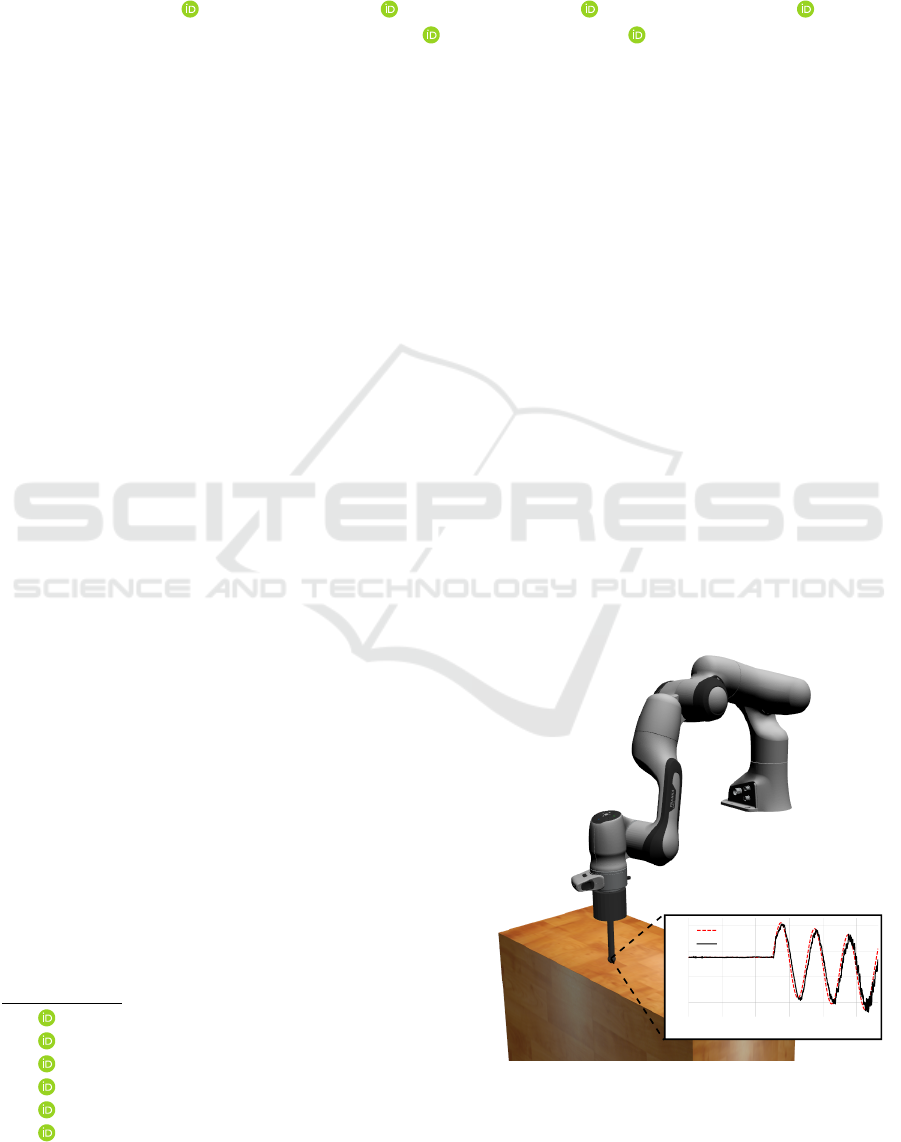
in a broad spectrum of tasks, including contact-rich
manipulation, precision assembly, and surface inter-
action (see Fig. 1).
To address this challenge, impedance controllers
achieve force-tracking accuracy through strategies
such as reference generation (Roveda and Piga, 2021;
Huang et al., 2022; Yu et al., 2024), variable stiff-
ness (Shen et al., 2022; Li et al., 2023), and variable
a
https://orcid.org/0009-0001-2295-0723
b
https://orcid.org/0000-0003-4777-1761
c
https://orcid.org/0000-0003-0768-8541
d
https://orcid.org/0000-0003-3385-8866
e
https://orcid.org/0000-0002-0476-4118
f
https://orcid.org/0000-0002-4427-536X
0 2 4 6 8 10
Time [s]
25
30
35
40
Force [N]
reference
actual
Figure 1: Simulation setup — the Panda robot performs
a force-tracking task sliding on a wooden table with a
spherical-tip end-effector.
394
Saad, K., Petrone, V., Ferrentino, E., Chiacchio, P., Braghin, F. and Roveda, L.
Augmenting Neural Networks-Based Model Approximators in Robotic Force-Tracking Tasks.
DOI: 10.5220/0013830700003982
Paper published under CC license (CC BY-NC-ND 4.0)
In Proceedings of the 22nd International Conference on Informatics in Control, Automation and Robotics (ICINCO 2025) - Volume 2, pages 394-401
ISBN: 978-989-758-770-2; ISSN: 2184-2809
Proceedings Copyright © 2025 by SCITEPRESS – Science and Technology Publications, Lda.

damping (Jung et al., 2004; Shu et al., 2021; Duan
et al., 2018; Roveda et al., 2020). Reference gen-
eration methods implement an explicit direct force
control (DFC) loop to follow a desired force trajec-
tory, while variable impedance approaches often rely
on simplified linear-spring environment models (Jung
et al., 2004; Shen et al., 2022; Li et al., 2023; Shu
et al., 2021; Duan et al., 2018; Yu et al., 2024). How-
ever, these simplified models typically represent only
an approximation of the real environment dynamics
(Roveda and Piga, 2021; Jung et al., 2004; Matschek
et al., 2023).
To overcome modeling inaccuracies, recent liter-
ature has explored Artificial Intelligence (AI) tech-
niques (Matschek et al., 2023), particularly Neural
Networks (NNs), to learn a model-less, data-driven
mapping between the manipulator’s end-effector state
and the exerted contact force directly at the control
level. In this context, ORACLE (Petrone et al., 2025)
was proposed as a controller that leverages NN-based
models to optimize force tracking. However, OR-
ACLE’s original formulation neglects the effects of
end-effector velocities tangential to the contact plane,
potentially limiting its prediction accuracy and track-
ing performance, especially at high velocities.
This paper presents an extension of the ORA-
CLE strategy by augmenting its model approxima-
tor’s state with tangential velocity components, result-
ing in a refined controller named Velocity-Augmented
Artificial Intelligence interaction Controller for Am-
biguous Models (VAICAM). The proposed approach
constructs an accurate model of the environment that
relates the end-effector pose, penetration velocity, and
tangential velocity to the resulting contact forces us-
ing feed-forward neural networks (FFNNs) (Naga-
bandi et al., 2018).
To this aim, a dedicated dataset containing dy-
namic trajectories in both force and position space
is generated to train this model effectively. An im-
proved controller is then designed based on this aug-
mented model, enabling optimal selection of con-
trol actions to minimize force-tracking errors. Ex-
tensive validation is carried out in simulation, using
Gazebo (Koenig and Howard, 2004), on a Franka
Emika Panda manipulator (Haddadin et al., 2022).
Furthermore, the paper conducts a comparative analy-
sis between a standard direct force controller (Roveda
and Piga, 2021) and ORACLE (Petrone et al., 2025)
across varying velocity conditions, concretely attest-
ing ORACLE’s performance degradation as the end-
effector velocity increases.
By integrating tangential velocity information into
the ORACLE framework, VAICAM demonstrates
improved force prediction and enhanced tracking
capabilities, extending the applicability of neural-
network-based force controllers to a wider range of
challenging interaction tasks.
2 METHODOLOGY
This paper introduces VAICAM, an AI-driven tool
to enhance the force tracking capabilities of an
impedance controller used in unknown environments.
It augments the ensemble of FFNNs originally pro-
posed in ORACLE (Petrone et al., 2025) by adding to
its input the tangential velocity v of the end-effector
(EE), resulting in a mapping from the robot state and
the DFC control action x
x
x
f
into its next state. This de-
sign choice yields a more accurate prediction of the
next wrench, that will later be used to compute the
optimal residual action added to the low-level control
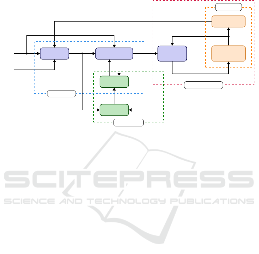
action of the DFC. VAICAM’s overall control scheme
is summarized in Fig. 2, whose building blocks will
be detailed in the next sections.
2.1 Base Controller
The low-level impedance controller enforces the de-
sired interaction dynamics on the robot, specifically,
Cartesian space mass-spring-damper dynamics. Con-
sider the equations of motion for a manipulator with
n Degrees of Freedom (DOFs) performing an m-
dimensional task, with m ≤ 6 ≤ n (Featherstone and
Orin, 2016):
B
B
B(q
q
q)
¨
q
q
q +C
C
C(q
q
q,
˙
q
q
q)
˙
q
q
q + τ
τ
τ
f
(
˙
q
q
q) + g
g
g(q
q
q) = τ
τ
τ
c
− J
J
J
⊤
(q
q
q)h
h
h
e
,
(1)
where B
B
B(q
q
q) ∈ R
n×n
is the inertia matrix, C
C
C(q
q
q,
˙
q
q
q) ∈
R
n×n
is the matrix accounting for the centrifugal and
Coriolis effects, τ
τ
τ
f
(
˙
q
q
q) ∈ R
n
accounts for viscous and
static friction, g
g
g(q
q
q) ∈ R
n
represents the torque exerted
on the links by gravity, τ
τ
τ
c
∈ R
n
indicates the torque
control action, J
J
J(q
q
q) ∈ R
m×n
is the geometric Jaco-
bian, and h
h
h
e
∈ R
m
is the vector of wrenches exerted on
the environment measured by means of a force/torque
sensor mounted on the manipulator’s flange. The vec-
tors q
q
q,
˙
q
q
q,
¨
q
q
q ∈ R
n
represent joint positions, velocities,
and accelerations, respectively.
The expression of the Cartesian impedance con-
trol law with robot dynamics compensation is (Sicil-
iano and Villani, 1999; Formenti et al., 2022)
τ
τ
τ
c
= J
J
J
⊤
(q
q
q)h
h
h
c
+C
C
C(q
q
q,
˙
q
q
q)
˙
q
q
q + τ
τ
τ
f
(
˙
q
q
q) + g
g
g(q
q
q), (2)
where the task space wrench h
h
h
c
realizing the compli-
ant behavior can be chosen as (Caccavale et al., 1999;
Iskandar et al., 2023)
h
h
h
c
= K
K
K
d
∆
∆
∆x
x
x + D
D
D
d
˙
x
x
x, (3)
Augmenting Neural Networks-Based Model Approximators in Robotic Force-Tracking Tasks
395
DFC (4) VAICAM (10)
Impedance
control (2)
Robot
dynamics (1)
Environment
MA (7)
Dataset
h
h
h
r
x
x
x
f
x
x
x
∗
c
τ
τ
τ
c
x
x
x,
˙
x
x
x
h
h
h
e
x
x
x
r
x
x
x
f
± ρ
ρ
ρ
ˆ
h
h
h
e
δ
δ
δ
ˆ
s
s
s =
ˆ
F (s
s
s,x
x
x
f
) − s
s
s
On-line control
Physical plant
Dynamical system F
Off-line training
s
s
s
Figure 2: Control architecture. The MA learns the transition function
ˆ
F of the dynamical system represented by the
impedance-controlled robot interacting with an unknown environment, given data composed of the system states s
s
s and control
inputs x
x
x
f
, i.e. the DFC action. After training, VAICAM computes the optimal residual action x
x
x
∗
c
, aiming at minimizing the
force tracking error between h
h
h
r
and the predicted wrench
ˆ
h
h
h
e
.
where K
K
K
d
,D
D
D
d
∈ R
m×m
are diagonal matrices of con-
trol parameters, namely stiffness and damping, re-
spectively, and ∆
∆
∆x
x
x ≜ x
x
x
d
− x
x
x ∈ R
m
is the Cartesian
pose error between the setpoint x
x
x
d
∈ R
m
and the ac-
tual robot pose x
x
x ∈ R
m
. Assuming m = 6, x
x
x is defined
as x
x
x ≜ (x,y, z, φ, θ, ψ)
⊤
, where (x, y,z)
⊤
and (φ,θ,ψ)
⊤
are translational and rotational components, respec-
tively.
2.2 Direct Force Controller
Given that the impedance controller solely manages
interaction forces passively, lacking the capability to
track a force reference, a DFC loop can be closed
specifically along the directions in which force track-
ing is necessary (Roveda and Piga, 2021). The
adopted control law is a simple PI controller having
the following model:
x
x
x
f
= x
x
x
r
+ Γ
Γ
Γ
K
K
K
P
∆
∆
∆h
h
h + K
K
K
I
Z
t
∆
∆
∆h
h
hdt
, (4)
where, if m = 6, Γ
Γ
Γ = diag(γ
x
,γ
y
,γ
z
,γ
φ
,γ
θ
,γ
ψ
) is the
task specification matrix (Khatib, 1987), with γ
i
= 1
if the i-th direction is subject to force control, 0 other-
wise. x
x
x
f
∈ R
m
is the force controller output, while
x
x
x
r
∈ R
m
is the reference pose, whose i-th compo-
nent is tracked when γ
i
= 0. K
K
K
P
,K
K
K
I
∈ R
m×m
are the
proportional and integral gains of the controller, and
∆
∆
∆h
h
h = h
h
h
r
− h
h
h
e
∈ R
m
is the error between the reference
wrench to be exerted h
h
h
r
∈ R
m
and the actual exerted
wrench h
h
h
e
∈ R
m
.
2.3 Model Approximator
The Model Approximator (MA) addresses the inher-
ent complications in accurately modeling the robot-
environment interaction with a rather straightforward
method that only requires the user to set up a handful
of experiments that autonomously train the NN-based
model. The MA deals with the current system state
s
s
s
k
, aiming to predict the state at the next time step
k + 1 following the equation
ˆ
s
s
s
k+1
=
ˆ
F (s
s
s
k
,x
x
x
f
), (5)
where
ˆ
s
s
s
k+1
is the predicted next state.
ˆ
F represents
the transition dynamics approximation which outputs
the next predicted state, where F indicates the ac-
tual dynamical system, i.e. the impedance-controlled
robot (see Fig. 2). Specifically, instead of predicting
s
s
s
k+1
explicitly, the actual FFNN’s output δ
δ
δ
ˆ
s
s
s is chosen
to be the approximate difference between two subse-
quent states, similarly to (Nagabandi et al., 2018), i.e.:
δ
δ
δs
s
s = s
s
s
k+1
− s
s
s
k
. (6)
This allows (5) to be rewritten as
ˆ
s
s
s
k+1
= s
s
s
k
+ δ
δ
δ
ˆ
s
s
s(s
s
s
k
,x
x
x
f
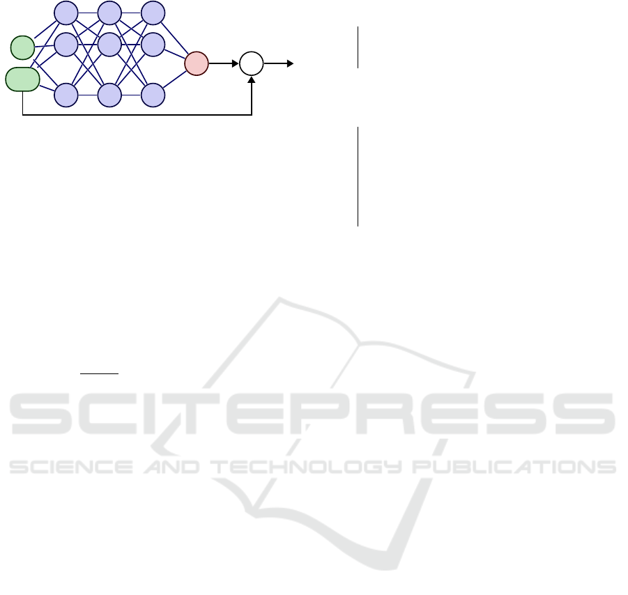
), (7)
with δ
δ
δ
ˆ
s
s
s(s
s
s
k
,x
x
x
f
) being the actual NN output, as in
Fig. 3.
As regards the state definition, in general s
s
s takes
the form
s
s
s ≜ (x
x
x,
˙
x
x
x,h
h
h
e
)
⊤
, (8)
ICINCO 2025 - 22nd International Conference on Informatics in Control, Automation and Robotics
396
x
x
x
f
s
s
s
k
(9)
.
.
.
.
.
.
.
.
.
δ
δ
δ
ˆ
s
s
s
input
layer
hidden layers
ˆ
F
output
layer
+
ˆ
s
s
s
k+1
Figure 3: MA architecture. The hidden layers approximate
the dynamics transition function s
s
s
k+1
= F (s
s
s
k
,x
x
x
f
) by pre-
dicting the state variation δ
δ
δ
ˆ
s
s
s.
but it might be specialized according to the task setup.
Indeed, assuming tracking forces only along the z
axis, ORACLE (Petrone et al., 2025) only considers
orthogonal components in s
s
s, i.e. EE penetration ve-
locity and force along the same direction. This work
introduces a new feature in s
s
s, namely the EE tan-
gential velocity v, which influences the evolution of
the exerted force, especially at high speeds (Iskandar
et al., 2023). In summary, we propose the following
augmentation in the MA state representation:
s
s
s ≜ (z, ˙z, f
z
)
⊤
→ s
s
s ≜ (z, ˙z,v, f
z
)
⊤
, (9)
where v =
p
˙x
2
+ ˙y
2
is the tangential velocity, with
˙x, ˙y being the velocity components on the EE xy plane,
and f
z
is the normal force along z, i.e., the contact
direction.
From an architectural standpoint, the FFNN is ac-
tually an ensemble of FFNN as in (Chua et al., 2018),
since using an array of N independently trained NNs
minimizes the errors risen by epistemic and stochastic
uncertainties.
2.4 VAICAM Algorithm
Acting as the glue that joins all items together,
the VAICAM algorithm combines the DFC-enhanced
impedance controller and the MA. It utilizes the con-
trol action output by the DFC x
x
x
f
along with the force
prediction of the MA
ˆ
h
h
h
e
, and then outputs the opti-
mal residual action x
x
x
∗
c
that will then be added to the
impedance controller action aiming at minimizing the
force tracking error. VAICAM will search for x
x
x
∗
c
in
the neighborhood of x
x
x
f
in an area centered around it
with predefined radius ρ
ρ
ρ > 0
0
0.
Then, the control input to the impedance con-
troller is updated by solving an optimization problem,
run at each control step k:
x
x
x
∗
c
(k) = argmin
x
x
x
c
∈x
x
x
f
±ρ
ρ
ρ
L
k
(s
s
s,x
x
x
c
,h
h
h
r
), (10)
where
L
k
(s
s
s,x
x
x
c
,h
h
h
r
) = |h
h
h
r
(k) −
ˆ
h
h
h
e
(s
s
s
k
,x
x
x
c
)| + Ω
k
(x
x
x
c
) (11)
Data: x
x
x
f
from (4), s
s
s = (x
x
x,
˙
x
x
x,h
h
h
e
)
⊤
,h
h
h
r
Result: x
x
x
∗
c
if k = 1 then
Set α
α
α, β
β
β and ρ
ρ
ρ;
Set weights of the pre-trained MA NN
ensemble;
end
Build the discretized neighborhood of candidate
optimal actions B
B
B
ρ
ρ
ρ
(x
x
x
f
) = [x
x
x
f
± ρ
ρ
ρ];
for x
x
x
c
∈ B
B
B
ρ
(x
x
x
f
) do
Infer the predicted force from the model
approximator with (7):
ˆ
h
h
h
e
(s
s
s,x
x
x
c
) = h
h
h
e
+ δ
δ
δ
ˆ
h
h
h
e
(s
s
s,x
x
x
c
);
Compute the regularizer in (12) as
Ω
k
(x
x
x
c
) = ∥x
x
x
c
∥
2
α
α
α
+ |x
x
x
c
− x
x
x
∗
c
(k − 1)|
β
β
β
;
Compute the corresponding loss function in
(11) as L
k
(s
s
s,x
x
x
c
,h
h
h
r
) = |h
h
h
r
−
ˆ
h
h
h
e
| + Ω
k
(x
x
x
c
);
end
Call VAICAM by solving the optimization
problem in (10) minimizing (11):
x
x
x
∗
c
(k) = argmin
x
x
x
c
∈B
B
B
ρ
ρ
ρ
(x
x
x
f
)
L
k
(s
s
s,x
x
x
c
,h
h
h
r
);
Algorithm 1: VAICAM algorithm at every control
step k.
is the cost function to minimize, whose first term |h
h
h
r
−
ˆ
h
h
h
e
| is the expected force tracking error, and
Ω
k
(x
x
x
c
) = ∥x
x
x
c
∥
2
α
α
α
+ |x
x
x
c
− x
x
x
∗
c
(k − 1)|
β
β
β
(12)
is a regularizer that contributes to smoothing-out large
jumps of the control term x
x
x
c
. The first term in (12) pe-
nalizes heavy actions so as to avoid deep penetrations
of the EE into the environment, whereas the second
prevents fast variations between subsequent actions.
The two terms are defined as:
∥x
x
x
c
∥
2
α
α
α
=
∑
i
α
i
x
2
c,i
, (13a)
|x
x
x
c
− x
x
x
∗
c
(k − 1)|
β
β
β
=
∑
i
β
i
|x
c,i
− x
∗
c,i
(k − 1)|, (13b)
where both α
α
α,β
β
β ∈ R
m
are parameters to be chosen by
the user. This method, summarized in Algorithm 1,
along with the base force controller, is activated as
soon as contact is established between the EE and the
environment.
2.5 Training Procedure
The training and validation of the ensemble of FFNN,
which is done in a preliminary offline stage, uses col-
lected data resulting from thorough exploration of the
state space. In order to collect the data, reference
forces and positions are provided to the base force
controller, and the output data, consisting of the ac-
tual robot states s
s
s and control actions x
x
x
f
, are recorded.
During the training stage of the FFNN, their weights
Augmenting Neural Networks-Based Model Approximators in Robotic Force-Tracking Tasks
397

are updated using the Stochastic Gradient Descent al-
gorithm in order to minimize the Mean Squared Error
(MSE) between the actual and estimated states.
In our training procedure, we recommend com-
manding sine waves as references in both force and
position spaces, in order to have a thorough explo-
ration and avoid data gaps in the state domain. Com-
manding a sine wave reference for the position addi-
tionally entails that the EE velocity v is sinusoidal,
allowing for the complete exploration of the velocity
space as well. This is a crucial aspect because, com-
pared to (Petrone et al., 2025), the inclusion of the
new feature v requires a dedicated training. Further-
more, we recommend exaggerating the amplitude of
the sine wave force references: even though they can-
not be perfectly tracked by the controller, this ensures
that the force domain is sufficiently explored.
After collecting data, they are then processed fol-
lowing methods used in (Nagabandi et al., 2018; Chua
et al., 2018), i.e. they are normalized by subtracting
the mean of each quantity and then dividing by its
standard deviation. A zero-mean Gaussian noise in
the form N (µ = 0,σ) is applied to the measured data
h
h
h
e
in order to enhance the robustness of the NN.
3 RESULTS
3.1 Task and Materials
The experimental validation is divided into two main
phases, both conducted on the 7-DOF Franka Emika
Panda robot:
• Experiment I: train, validate, and test the Static
Model Approximator (SMA) used by ORACLE,
which is the MA trained and validated using static
position references (Petrone et al., 2025) without
tangential velocity, and the Dynamic Model Ap-
proximator (DMA) used by VAICAM, which is
the MA trained and validated using dynamic posi-
tion references with tangential velocities;
– the goal is to assess the performance of both
MAs on dynamic position reference trajecto-
ries, and validate that the DMA yields higher
accuracy as the tangential velocity increases;
• Experiment II: execute dynamic trajectories us-
ing the base controller (Roveda and Piga, 2021),
ORACLE (Petrone et al., 2025) and VAICAM,
and compare the force tracking results;
– in this case, the objective is to assess the per-
formance of both control strategies, and val-
idate that the controller that uses the DMA
(VAICAM) performs better than both the base
Table 1: Parameters used in the experiments.
Parameter Value
Coulomb friction coefficient µ 0.2
Time step solver ODE
Impedance control translational stiffness K
d,t
1700
Impedance control orientational stiffness K
d,r
300
Damping ratio ξ 1
DFC Proportional gain K
P
1· 10
−6
DFC Integral gain K
I
2· 10
−3
Table 2: Configurations of the FFNN ensemble.
Parameter Value
Number of estimators N 3
Hidden layers 3
Neurons per layer 200
Activation function ReLU
Learning rate 1· 10
−3
Ensemble type Fusion
Training epochs 50
Loss function MSE
Weight optimizer Adam
controller and the controller that uses the SMA
(ORACLE).
The NN’s algorithm is coded in Python using
PyTorch (Paszke et al., 2019), interfacing with the
other modules via ROS communication mechanisms
(Quigley et al., 2009). The controllers implemented
in ROS are coded in C++.
In order to accurately simulate the robot,
Gazebo (Koenig and Howard, 2004) is used as
the simulation software. A spherical tip EE is
mounted at the flange of the robot (see Fig. 1).
The interaction control parameters are chosen as
K
K
K
d
= diag(K
d,t
,K
d,t
,K
d,t
,K
r,t
,K
r,t
,K
r,t
) and D
D
D
d
=
diag{ξ
p
K
d,i
}
6
i=1
, where K
d,t
and K
d,r
are the transla-
tional and rotational stiffness gains, respectively, and
ξ is the damping ratio. Table 1 provides a summary
of the parameters. In our experiment, a linear force is
exerted on the z axis, thus Γ
Γ
Γ = diag(0,0,1,0,0,0).
3.2 Experiment I: Model Approximator
Validation
For a fair comparison with (Petrone et al., 2025),
we base the FFNNs structure on the findings therein.
Specifically, all FFNNs used share the same config-
uration in terms of depth (number of hidden layers),
width (number of neurons per layer) and learning al-
gorithm parameters, as listed in Table 2. Linear type
layers are used, while the activation function is of the
ReLU type (Agarap, 2019). The optimized config-
uration of the base estimator that ensures enhanced
inference time without compromising prediction ac-
ICINCO 2025 - 22nd International Conference on Informatics in Control, Automation and Robotics
398
curacy uses N = 3 FFNNs. Adam (Kingma and Ba,
2015) refers to Adaptive Moment Estimation, an op-
timizer used for NN regression tasks, while “Fusion”
indicates how a single output is retrieved from the en-
semble, i.e. the arithmetic average across the indepen-
dent network estimations is computed.
3.2.1 Static Model Approximator
The dataset is composed of 10 trajectories, with 9 of
them being used in the training set, and the remain-
ing 1 in the validation set, used by Adam (Kingma
and Ba, 2015) to adaptively optimize the learning
rate. The position reference is in the form of a static
waypoint, as this MA, unlike the one proposed in
this work, does not take into consideration v (Petrone
et al., 2025). The force reference is in the form of
a sinusoidal wave with randomized frequency, ampli-
tude, and mean. Raw data in both training and valida-
tion sets are pre-processed as indicated in Sect. 2.5.
After training the MA, a test set is developed in
order to assess its performance. Since the aim of
this work is to assess the MA generalization ability
against dynamic position trajectories, this set is com-
posed of horizontal line references that the EE tries to
track with a constant velocity and a sinusoidal force
reference. The MA is tested against a total of 110 tra-
jectories of about 1.2m executed using the base con-
troller, divided into 11 evenly-spaced velocities in the
range [0.01,0.50]m/s. The performance assessment
is based on the comparison of the force predicted by
the MA with the actual force.
3.2.2 Dynamic Model Approximator
Compared to the SMA discussed in Sect. 3.2.1, we
adopt a different training approach, i.e. both the force
and position references in the training set take a si-
nusoidal form. On the basis of the training proce-
dure outlined in Sect. 2.5, sinusoidal position refer-
ences allow covering the desired velocity span bet-
ter than constant velocity profiles. The validation set
is composed of 11 trajectories, each randomly given
a velocity from the 11 velocity samples in the range
[0.01,0.50]m/s.
After executing the trajectories, the data stored in
the dataset are pre-processed according to the proce-
dure reported in Sect. 2.5. Using the DMA, the net-
work now takes into consideration v while predicting
the next state, which ameliorates the performance of
the MA at higher velocities. In order to confirm this
thesis, the DMA is evaluated on the same test set as
the SMA’s, i.e. using the same 110 line trajectories.
0.0 0.1 0.2 0.3 0.4 0.5
Velocity [m/s]
0.02
0.04
0.06
0.08
0.10
0.12
RMSE [N]
Dynamic MA
Static MA
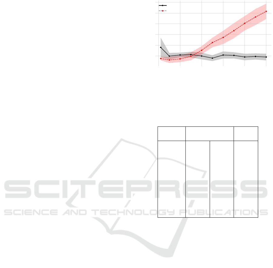
Figure 4: Comparison between the static and the dynamic
model approximators, in terms of RMSE, as the EE velocity
increases.
Table 3: Average RMSE of static and dynamic model ap-
proximators across trajectories — η indicates the improve-
ment factor of DMA over SMA.
Velocity RMSE [N]
η
η
η
[m/s] SMA DMA
0.01 0.0154 0.0397 0.3877
0.05 0.0135 0.0203 0.663
0.1 0.0155 0.022 0.7029
0.15 0.0203 0.0228 0.8893
0.2 0.0312 0.0207 1.511
0.25 0.0456 0.0165 2.7628
0.3 0.0557 0.0225 2.4777
0.35 0.0684 0.0216 3.1683
0.4 0.0819 0.0188 4.3528
0.45 0.0936 0.0196 4.7841
0.5 0.104 0.0188 5.5422
3.2.3 Model Approximators Comparison
Fig. 4 reports the Root Mean Square Error (RMSE)
between the predicted and measured force, when ei-
ther the SMA or DMA is employed, for increasing
EE tangential velocity v. As expected, the plot re-
veals a better generalization ability of the DMA over
the SMA to higher EE velocities. While the results
are comparable at low speed, as v increases the SMA
showcases lower prediction accuracy, in terms of both
mean and variance across trajectories.
This qualitative analysis is quantitatively con-
firmed by Table 3, which also reports the numerical
improvement factor η of DMA over SMA. As v in-
creases, the former outperforms the latter by up to
454%, in terms of average RMSE recorded across tra-
jectories at the same velocity.
Augmenting Neural Networks-Based Model Approximators in Robotic Force-Tracking Tasks
399

0.0 0.1 0.2 0.3 0.4 0.5
Velocity [m/s]
1
2
3
4
5
6
7
RMSE [N]
VAICAM
ORACLE
DFC
Figure 5: Comparison between the baseline DFC (Roveda
and Piga, 2021), ORACLE (Petrone et al., 2025), and
VAICAM (ours), in terms of RMSE, as the EE velocity in-
creases.
0 1 2 3 4 5 6 7 8
Time [s]
6
8
10
12
14
16
18
Force [N]
reference
ORACLE
VAICAM
±1 N error
Figure 6: Force tracking comparison between ORACLE
(Petrone et al., 2025) and VAICAM (ours) at v = 0.2m/s.
3.3 Experiment II: Control Algorithm
Validation
Once the SMA and the DMA are trained, the three
control algorithms — DFC (Roveda and Piga, 2021),
ORACLE (Petrone et al., 2025), and VAICAM (ours)
— can be tested against a test set aiming to prove that
VAICAM outperforms its competitors. The optimizer
parameters are tuned as α = 25, β = 200, and ρ =
0.003m for both ORACLE and VAICAM.
As can be seen from Fig. 5, the average force-
tracking RMSE for VAICAM is approximately con-
stant for v ∈ [0, 0.35] m/s, and starts increasing for
v > 0.35m/s. Thanks to the exploitation of the novel
DMA, VAICAM outperforms both ORACLE and the
base DFC. A sample trajectory is considered in Fig. 6,
visually showing that ORACLE’s uncertainty at mod-
erate velocities (due to the limited SMA) translates
into worse force-tracking capabilities. Furthermore,
Fig. 5 shows that VAICAM also enhances the DFC
performance, although with a lower improvement fac-
tor compared to ORACLE. Lastly, it is worth noticing
that VAICAM’s RMSE standard deviation is lower
than DFC’s, thus manifesting a superior robustness
w.r.t. the experimental conditions.
Table 4: Average RMSE of baseline DFC (Roveda and
Piga, 2021), ORACLE (Petrone et al., 2025), and VAICAM
(ours) across trajectories — η indicates the improvement
factor of VAICAM over DFC or ORACLE.
Velocity RMSE [N] η
η
η
[m/s] DFC ORACLE VAICAM DFC ORACLE
0.01 2.0579 2.1222 2.0676 0.9953 1.0264
0.05 2.0602 2.1867 1.8917 1.0891 1.1559
0.1 2.1022 2.2118 2.0259 1.0377 1.0918
0.15 2.1563 3.135 2.0528 1.0504 1.5272
0.2 2.199 3.5081 2.0697 1.0624 1.695
0.25 2.3638 3.8424 2.0362 1.1609 1.887
0.3 2.4995 4.3858 2.1098 1.1847 2.0788
0.35 2.6919 4.6601 2.0553 1.3097 2.2673
0.4 2.973 4.883 2.3837 1.2472 2.0485
0.45 3.1873 4.978 2.5117 1.269 1.982
0.5 3.3923 5.4201 2.8123 1.2062 1.9273
To confirm the improvement of VAICAM over
both DFC and ORACLE, Table 4 displays the numer-
ical results by reporting the average RMSE of these 3
strategies for each velocity. As η confirms, VAICAM
surpasses the DFC by up to 31% (at v = 0.35m/s),
while the improvement over ORACLE at maximum
experimental speed (v = 0.5m/s) reaches 127%.
4 CONCLUSIONS
This paper introduced VAICAM, a controller improv-
ing the state-of-the-art of robot-environment interac-
tion tasks that require dynamic trajectories. It makes
use of an FFNN ensemble that acts as a model approx-
imator considering the tangential velocity of the EE.
The controller is based on an impedance controller to
ensure a compliant behavior, and a DFC to guarantee
the desired force tracking characteristics. An ensem-
ble of FFNNs is developed, trained, and tested along
the work. The networks are able to predict the force
that the manipulator will exert on the environment,
allowing the computation of an optimal residual ac-
tion. The latter is then added to the action of a base-
line DFC to improve its force-tracking capabilities, by
correcting the next commanded position. Tested in a
simulated environment, VAICAM outperformed the
baseline DFC (Roveda and Piga, 2021) and a similar
algorithm from recent literature (Petrone et al., 2025).
Possible future improvements of the proposed
strategy are: (i) extending the comparison with other
controllers from the literature, e.g. (Iskandar et al.,
2023); (ii) assessing whether these controllers can
benefit from a MA like the one developed in this
work to improve their performance; (iii) deploying
the algorithm on real hardware, for a complete val-
idation of VAICAM’s performance; (iv) extending
the state space to include tangential position com-
ponents, to tackle variable-stiffness environments;
(v) including the DMA in optimal planning algo-
ICINCO 2025 - 22nd International Conference on Informatics in Control, Automation and Robotics
400

rithms foreseeing robot-environment interaction tra-
jectories (Petrone et al., 2022).
REFERENCES
Agarap, A. F. (2019). Deep Learning using Rectified Linear
Units (ReLU). arXiv preprint: 1803.08375.
Caccavale, F., Natale, C., Siciliano, B., and Villani, L.
(1999). Six-DOF impedance control based on an-
gle/axis representations. IEEE Trans. Robot. Au-
tomat., 15(2):289–300.
Chua, K., Calandra, R., McAllister, R., and Levine, S.
(2018). Deep Reinforcement Learning in a Handful
of Trials using Probabilistic Dynamics Models. In
Adv. Neural Inform. Process. Syst., volume 32, pages
4754–4765.
Duan, J., Gan, Y., Chen, M., and Dai, X. (2018). Adap-
tive variable impedance control for dynamic contact
force tracking in uncertain environment. Robot. Au-
ton. Syst., 102:54–65.
Featherstone, R. and Orin, D. E. (2016). Dynamics. In
Siciliano, B. and Khatib, O., editors, Springer Hand-
book of Robotics, volume 3, pages 195–211. Springer,
2 edition.
Formenti, A., Bucca, G., Shahid, A. A., Piga, D., and
Roveda, L. (2022). Improved impedance/admittance
switching controller for the interaction with a variable
stiffness environment. Compl. Eng. Syst., 2(3). Art.
no. 12.
Haddadin, S., Parusel, S., Johannsmeier, L., Golz, S.,
Gabl, S., Walch, F., Sabaghian, M., J
¨
ahne, C., Haus-
perger, L., and Haddadin, S. (2022). The Franka
Emika Robot: A Reference Platform for Robotics Re-
search and Education. IEEE Robot. Automat. Mag.,
29(2):46–64.
Huang, H., Guo, Y., Yang, G., Chu, J., Chen, X., Li, Z.,
and Yang, C. (2022). Robust Passivity-Based Dy-
namical Systems for Compliant Motion Adaptation.
IEEE/ASME Trans. Mechatron., 27(6):4819–4828.
Iskandar, M., Ott, C., Albu-Sch
¨
affer, A., Siciliano, B., and
Dietrich, A. (2023). Hybrid Force-Impedance Control
for Fast End-Effector Motions. IEEE Robot. Automat.
Lett., 8(7):3931–3938.
Jung, S., Hsia, T. C. S., and Bonitz, R. G. (2004). Force
Tracking Impedance Control of Robot Manipulators
Under Unknown Environment. IEEE Trans. Contr.
Syst. Technol., 12(3):474–483.
Khatib, O. (1987). A unified approach for motion and force
control of robot manipulators: The operational space
formulation. IEEE J. Robot. Automat., 3(1):43–53.
Kingma, D. P. and Ba, J. (2015). Adam: A Method for
Stochastic Optimization. In Int. Conf. Learn. Repre-
sent.
Koenig, N. and Howard, A. (2004). Design and Use
Paradigms for Gazebo, an Open-Source Multi-Robot
Simulator. In IEEE Int. Conf. Intell. Robots Syst., vol-
ume 3, pages 2149–2154.
Li, K., He, Y., Li, K., and Liu, C. (2023). Adaptive
fractional-order admittance control for force tracking
in highly dynamic unknown environments. Int. J.
Robot. Res. Applic., 50(3):530–541.
Matschek, J., Bethge, J., and Findeisen, R. (2023). Safe
Machine-Learning-Supported Model Predictive Force
and Motion Control in Robotics. IEEE Trans. Contr.
Syst. Technol., 31(6):2380–2392.
Nagabandi, A., Kahn, G., Fearing, R. S., and Levine, S.
(2018). Neural Network Dynamics for Model-Based
Deep Reinforcement Learning with Model-Free Fine-
Tuning. In IEEE Int. Conf. Robot. Automat., pages
7559–7566.
Paszke, A., Gross, S., Massa, F., Lerer, A., Bradbury, J.,
Chanan, G., Killeen, T., Lin, Z., Gimelshein, N.,
Antiga, L., Desmaison, A., K
¨
opf, A., Yang, E., De-
Vito, Z., Raison, M., Tejani, A., Chilamkurthy, S.,
Steiner, B., Fang, L., Bai, J., and Chintala, S. (2019).
PyTorch: An Imperative Style, High-Performance
Deep Learning Library. In Adv. Neural Inform. Pro-
cess. Syst., volume 33, pages 8026–8037.
Petrone, V., Ferrentino, E., and Chiacchio, P. (2022).
Time-Optimal Trajectory Planning With Interaction
With the Environment. IEEE Robot. Automat. Lett.,
7(4):10399–10405.
Petrone, V., Puricelli, L., Pozzi, A., Ferrentino, E., Chi-
acchio, P., Braghin, F., and Roveda, L. (2025). Op-
timized Residual Action for Interaction Control with
Learned Environments. IEEE Trans. Contr. Syst. Tech-
nol. Accepted for publication.
Quigley, M., Conley, K., Gerkey, B., Faust, J., Foote, T.,
Leibs, J., Wheeler, R., and Ng, A. (2009). ROS: an
open-source Robot Operating System. In IEEE Int.
Conf. Robot. Automat., volume 3.
Roveda, L., Castaman, N., Franceschi, P., Ghidoni, S., and
Pedrocchi, N. (2020). A Control Framework Defini-
tion to Overcome Position/Interaction Dynamics Un-
certainties in Force-Controlled Tasks. In IEEE Int.
Conf. Robot. Automat., pages 6819–6825.
Roveda, L. and Piga, D. (2021). Sensorless environ-
ment stiffness and interaction force estimation for
impedance control tuning in robotized interaction
tasks. Auton. Robots, 45(3):371–388.
Shen, Y., Lu, Y., and Zhuang, C. (2022). A fuzzy-based
impedance control for force tracking in unknown en-
vironment. J. Mech. Sci. Technol., 36(10):5231–5242.
Shu, X., Ni, F., Min, K., Liu, Y., and Liu, H. (2021).
An Adaptive Force Control Architecture with Fast-
Response and Robustness in Uncertain Environment.
In Int. Conf. Robot. Biom., pages 1040–1045.
Siciliano, B. and Villani, L. (1999). Indirect Force Control.
In Robot Force Control, pages 31–64. Springer US.
Yu, X., Liu, S., Zhang, S., He, W., and Huang, H. (2024).
Adaptive Neural Network Force Tracking Control of
Flexible Joint Robot With an Uncertain Environment.
IEEE Trans. Ind. Electron., 71(6):5941–5949.
Augmenting Neural Networks-Based Model Approximators in Robotic Force-Tracking Tasks
401
