Research on the Current Situation of Intergenerational Income Flow

and Its Influencing Mechanism

Yuexia Zhang

Institute of Quantitative Economics and Statistics, Huaqiao University, Xiamen, 361021, China

Keywords: Intergenerational Mobility, Influencing Mechanism, Multiple Linear Regression.

Abstract: As socialism with Chinese characteristics enters a new era, further deepening reform requires breaking

through the barriers of solidified interests. It is essential to analyze the current situation of inter-generational

income flow, explore the causes of inter-generational income flow. The research first consulted the population

of each administrative region of Xiamen City through the seventh population census data, conducted multi-

stage sampling. It conducted a qualitative and quantitative investigation of the existing state of

intergenerational income flow using a questionnaire survey. Thus, three features of the current state of

intergenerational income flow were obtained: Parents' assistance in children's growth, education and

employment, individuals' views on intergenerational income flow, and their cognition of income comparison.

Then, based on the multiple linear regression model, the influence mechanism of the child income is analyzed.

Additionally, the income elasticity across generations is determined. The findings indicate that the study's

contents have a favorable effect on the offspring's intergenerational income.

1 INTRODUCTION

The primary focus of social mobility research is

intergenerational mobility. Intergenerational income

mobility (IIM) refers to the relationship or elasticity

of children's income to that of their parents. The

situation can reflect the basic order and opportunity

structure of the society as well as the relationship

model between different classes, so it has been paid

much attention.

IIM was mainly studied about human capital

(Becker & Thomes, 1979). At first, in order to

accurately measure IIM, many scholars studied

temporary income bias. Life cycle bias and co-

resident sample bias are used to correct

intergenerational mobility.

To address the issue of temporary income bias,

combined with the theory of permanent income and

reduced the bias caused by short-term fluctuations by

taking the average years of the current income of the

parents as the proxy variable of permanent income

(Solon et al., 1992). Bjorklund corrected the upward

bias of intergenerational income elasticity based on

Solon by using the father's years of education and

https://orcid.org/0009-0007-1690-2745

occupation as instrumental variables (Bjorklund et al.,

1997). About the correction of life cycle bias, Haier

found that the actual income in the early 30s and mid-

40s was used to estimate the minimum bias and was

most suitable for estimating the average income close

to the lifetime (Haider et al., 2006). Co-living sample

selection bias, that is, co-living sample in the same

family can easily lead to high estimation of

intergenerational income elasticity. At present, the

proportion of parents living with their children in

China is gradually declining, and most of the existing

databases conduct unified surveys based on the family

level, which is easy to lead to the situation of

respondents asking more questions than answers,

resulting in large intra-sample bias.

Based on gradually improving the correction of

the bias of income indicators, Dahl proposed to use

the correlation coefficient of intergenerational income

rank as a new measurement index to describe the

intergenerational income relationship (Dahl et al.,

2008). C&H introduced quantile regression of

instrumental variables to further eliminate its bias

(Chernozhukov & Hansen, 2008). Zhang deeply

discussed the impact of education level on the

Zhang, Y.

Research on the Current Situation of Intergenerational Income Flow and Its Inﬂuencing Mechanism.

DOI: 10.5220/0013829400004708

Paper published under CC license (CC BY-NC-ND 4.0)

In Proceedings of the 2nd International Conference on Innovations in Applied Mathematics, Physics, and Astronomy (IAMPA 2025), pages 557-566

ISBN: 978-989-758-774-0

557

intergenerational transmission of relative poverty in

rural families (Zhang, 2024). Wang sorted out and

summarized the research results on intergenerational

income mobility (Wang Shanshan, 2023). Levi found

that the ability of education to regulate inter-

generational mobility is limited (Levi, 2018), just as

Chen thought that the expansion of higher education

has reduced its value (Chen, 2023). Shu demonstrated

how the opening up and restructuring of the economic

system have undermined the value transformation of

education (Shu, 2022).

Through questionnaire design and investigation,

the paper carries out factor analysis after data

differentiation analysis, reliability analysis and

validity analysis, and explores the causes of inter-

generational income flow by analyzing the current

situation (CS) of inter-generational income flow and

multiple linear regression model, and puts forward

constructive suggestions.

2 INVESTIGATION METHOD

2.1 Questionnaire Survey Method

The research group conducted two questionnaire

surveys, namely pre-survey and formal survey. The

questionnaire was randomly sampled and distributed

using the questionnaire star platform. After clearing

the faulty surveys, the pre-investigation yielded 62

valid questionnaires, while the official investigation

yielded 150 valid questionnaires.

The questionnaire used in this survey is set into

three sections: the basic information of the

respondents, the situation of the respondents' parents,

and the factors affecting the intergenerational income

flow.

2.1.1 Questionnaire Content Design

In the first step, it determines the topic direction

according to the research content: analysis of the CS

of intergenerational income flow and its influence

mechanism. In the second step, it consulted relevant

literature and books according to the direction of topic

selection, carried out field investigation in Xiamen,

collected relevant information, and further

understood the relevant situation. The third step is to

design different types of questions according to the

situation of field investigation and enrich the contents

of the questionnaire.

2.1.2 Modification and Improvement of the

Questionnaire

After the questionnaire was designed and completed,

the content, wording, format and sequence of the

questionnaire were analyzed several times, and the

questionnaire was adjusted and modified to make it

more concise and substantial, to better obtain the

information needed for the survey.

2.2 Multi-Stage Sampling

This research group adopts multi-stage sampling, and

the sampling process is carried out in stages. Different

sampling methods are used in each stage, that is,

various sampling methods are combined to consider

not only the sample representativeness, but also the

manpower required and the total cost incurred in

issuing questionnaires.

3 SURVEY DATA ANALYSIS

3.1 Differentiation Analysis

The primary purpose of item analysis is to delete

items with low differentiation degree. After

recovering the pre-survey questionnaire, the research

team first selects effective questionnaires and

analyzes the differentiation degree of scale items in

the questionnaire. The purpose is to study whether the

data can effectively distinguish between high and low

levels, to evaluate the quality of a specific item. The

total scores of all respondents were ranked in high

order. From the analysis results, it can be seen that the

score of the high group is above 42 points, and the

score of the low group is below 25 points. The test

results of 10 items in the scale are all significant

(P<0.05). The final result shows that all items in the

scale have differentiation and can identify different

interviewees.

3.2 Reliability Analysis

Reliability analysis is to prove the reliability of the

research sample data through analysis, which can be

divided into four categories:

coefficient,

broken half reliability, duplicate reliability and retest

reliability. Since multiple measurements were not

made in this pre-survey, the internal uniform

convergence coefficient

was adopted to

test the reliability of the data in consideration of the

reliability analysis. The calculation formula of the

coefficient is shown:

IAMPA 2025 - The International Conference on Innovations in Applied Mathematics, Physics, and Astronomy

558





=−

−







(1)

Where

is the total number of questions in the

scale,

denotes the

𝑖

th in-question variance, and

is the variance of the total score of all items. The

coefficient

evaluates the internal

consistency of the scores of each survey item in the

scale question. Generally speaking, the coefficient

is best above 0.8, and 0.7-0.8 is an

acceptable range. If the coefficient is below 0.6, the

scale needs to be reconsidered.

The questionnaire was divided into five

dimensions: health status, education concept, CS

view, income comparison, and family help, and the

coefficients

were calculated by SPSS

analysis software to judge their reliability level. The

output is shown in Table 1.

Table 1:

Pre-survey Coefficients

Dimensions

Coefficient

Number of terms Evaluation result

Health status 0.838 2 Good reliability

Educational concept 0.712 2 Good credibility

Status quo view 0.776 2 Reliability is good

Income comparison 0.844 2 Good reliability

Home help 0.719 2 Good reliability

Scale overall 0.821 10 Good reliability

3.3 Validity Analysis (VA)

VA is to continue to analyze the validity of the item

after completing the reliability analysis. There are

many kinds of VA, and the VA of the pre-survey

questionnaire can usually be divided into content VA

and structural VA. Exploratory factor analysis (EFA)

and confirmatory factor (CFA) were used to analyze

the validity of the questions.

Firstly, the EFA was carried out, which was a

cyclic exploration process. The research group used

Bartlett sphericity (BS) test and KMO test on the

scale, the purpose of which was to test whether the

questionnaire items and factors had a good

correspondence.

For BS test, check whether its value is less than

0.05. If the value is less than 0.05, it means that BS

test is passed. For KMO test, check whether its KMO

value is greater than 0.6, if the KMO value is greater

than 0.6, it indicates that it is suitable for exploratory

factor analysis, and the larger the value, the better.

The output results of SPSS are shown in Table 2:

Table 2: Pre-investigated KMO and BS tests

Adequacy test KMO test 0.831

BS test

Approximate Chi-square 1335.116

Degrees of Freedom 378

value

0.000

As can be seen from Table 2, KMO value is 0.831

and BS test value

is less than 0.05, which is

significant, indicating that the questionnaire scale is

suitable for factor analysis.

When factor extraction was carried out by the

principal component analysis method, the number of

factors to be extracted was set to 5 due to the research

dimensions of 5 when designing the scale, and the

results were rotated by variance orthogonal. At the

same time, the display format of factor load

coefficients was set to form a matrix according to the

order of size, and variables with load coefficients less

Research on the Current Situation of Intergenerational Income Flow and Its Inﬂuencing Mechanism

559

than 0.4 were excluded. The variables

with higher load on the same factor are grouped

together, so as to better observe the corresponding

relationship between factors and items and get a

conclusion. The output result of total variance

interpretation is shown in T

able 3, and the factor load matrix obtained after

orthogonal rotation is shown in Table 4:

Table 3: Total variance interpretation table

Compon

ents

Initial eigenvalues

Extract the sum of squares of

loads

Rotate the load sum of squares

total

Variance

(%)

Cumula

tive (%)

Total

Variance

(%)

Cumulati

ve (%)

Total

Varianc

e (%)

Cumulativ

e (%)

1 10.015 35.766 35.766 10.015 35.766 35.766 5.15 18.392 18.392

2 2.6 9.285 45.052 2.6 9.285 45.052 3.298 11.779 30.171

3 2.347 8.382 53.434 2.347 8.382 53.434 3.294 11.763 41.934

4 1.654 5.906 59.34 1.654 5.906 59.34 2.922 10.437 52.371

5 1.262 4.508 74.054 1.262 4.508 74.054 1.41 5.035 74.054

Table 4: Composition matrix after rotation

Ingredients

1 2 3 4 5 6 7

Mental health status 0.666

Physical health 0.791

The degree to which an individual

values education

0.784

The degree to which one's parents

value education

0.693

Agree that "a poor family cannot

produce a noble son"

0.602

"Knowledge changes destiny" 0.865

Income versus peers 0.622

Compare your income to that of your

parents

0.853

The extent to which the income gap is

influenced by the family

0.838

The extent to which parents help with

employment

0.699

According to the requirement of factor load in

factor analysis, if the total variation rate of principal

factor explanation is greater than 60% and the factor

load is greater than 0.6, then the structural validity is

good. From the observation of Table 3, it can be seen

that the accumulated variance explanation rate of the

five factors extracted is 74.054%, and the factor load

of the 10 indicators studied is greater than 0.6,

indicating that the factors can extract the information

of each item well, and the convergent and

discriminative validity of the scale meet the relevant

requirements. Further observe the rotation component

matrix in Table 4. The corresponding relationship

between the five factors extracted and the items was

consistent with the expectation.

3.4 Formal Questionnaire Data

Processing and Testing

This data review primarily uses a manual format that

is broken down into two phases: The first step is to

confirm the questionnaire's thoroughness by

reviewing it soon after the survey, correctness, and

consistency. Considering that the survey subjects

come from all walks of life and have different

educational backgrounds, whether the questionnaire

content is clear and easy to understand is also the key

to consider; In the second stage, I audited all

questionnaires after completing all questionnaire

distribution tasks, to ensure the consistency of

processing methods. After first examination, 849 of

IAMPA 2025 - The International Conference on Innovations in Applied Mathematics, Physics, and Astronomy

560

the 886 questionnaires that were distributed for this

study were recovered, yielding a 95.8% recovery rate.

After finishing the questionnaire, the specific

coding method was as follows: the question number

was set as Q1, Q2, Q3…. The function of calculating

variables refers to a mathematical transformation that

deals with the items in the questionnaire. This

function is usually used in two situations in

questionnaire research, namely, variable production

and variable processing. The four items Q10, Q26,

Q27, Q28, and Q29 were respectively calculated and

the data columns generated were named as "health

level", "education concept", "CS view", "income

comparison" and "family help".

For missing, duplicate, incomplete and other

questionnaire data, data cleaning, for a small number

of missing values will be replaced by the mean of the

same category, and for a large number of missing

values of the questionnaire will not be investigated

and analyzed, that is, scrapped.

3.5 Data Inspection

3.5.1 Random Run Test

Random run test uses the run to construct the Z

statistic and gives the corresponding associated

probability value according to the normal distribution

table. The test results were shown in Table 5, all

values were greater than 0.05, and the null hypothesis

was not rejected. Therefore, the questionnaire

samples could be considered as random samples and

could be analyzed in the following data.

Table 5: Run test table

Fitness Level

Educational

perception

Z -0.711 0.512

value

0.477 0.608

3.5.2 Reliability Test

The test method and process of the reliability of the

formal questionnaire are the same as those of the pre-

survey, and the results show that the

coefficients at all levels are shown in Table 5.

Table 6:

The coefficients of the formal survey

Dimensions

Coefficient

Number of terms Evaluation results

Health status 0.838 2 Good reliability

Educational concept 0.712 2 Good credibility

Status quo view 0.776 2 Reliability is good

Income comparison 0.844 2 Good reliability

Home help 0.719 2 Good reliability

Scale ensemble 0.821 10 Good reliability

The results show that the

coefficients of all dimensions are greater than 0.7, and

the

coefficient of the scale as a whole is

0.821, which indicates that the internal consistency of

the questionnaire is good, and the scientific and

rational design of the questionnaire structure and

questions meet the requirements of market research

and analysis in this line.

3.5.3 Validity Test

The concept and basic theory of questionnaire

validity test have been mentioned in the pre-survey

data analysis, so it will not be repeated. In the same

process as the pre-survey validity test, KMO test and

BS test are first performed. The calculated KMO

value is 0.893 and greater than 0.7, and the

corresponding

value of BS test is less than 0.05, as

shown in Table 7.

TABLE7. Formal investigation of KMO and BS test

Adequacy test KMO test 0.893

Approximate Chi-

square

2893.846

Degrees of

Freedom

378

value

0.000

Research on the Current Situation of Intergenerational Income Flow and Its Inﬂuencing Mechanism

561

4 CURRENT ANALYSIS OF

INTERGENERATIONAL

INCOME FLOWS

Through the analysis of parents' help in children's

growth, education and employment, individuals'

views on intergenerational income flow and their own

cognition of income comparison, the main direction

of this investigation is determined.

4.1 The Analysis of Parents' Help to

Their Children

4.1.1 The Help Parents Provide to Their

Children's Development

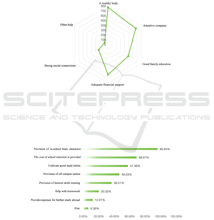
Figure 1: Parents' assistance in the development of their children (Photo/Picture credit: Original).

First of all, the article surveyed the help provided by

parents in the growth of their children, as shown in

Figure 1. Among the surveyed people, the help

received from parents comes from many aspects,

including economic, educational, spiritual, physical,

and other aspects, and is not limited to financial

support, which shows that in today's society, parents

take into account the cultivation of their children in

many aspects. At all levels of the survey, almost all

respondents agreed that they get good health from

their parents, while more than half of respondents

acknowledged that they get good company, adequate

financial support and good family education.

4.1.2 Parents' Help with Their Children's

Education

Figure 1: Parents' help with their children's education (Photo/Picture credit: Original).

Secondly, the research team made statistics on the

help provided by parents in the child's education. As

shown in Figure 2, almost all of the respondents'

parents provide for their basic education in school,

which is consistent with our cognition. In addition,

more than half of the respondents, 68.67% and

IAMPA 2025 - The International Conference on Innovations in Applied Mathematics, Physics, and Astronomy

562

57.36%, pay for school choice and cultivate their

children's good study habits, respectively. At the

same time, 46.53% of the respondents said that their

parents would provide the expenses for after-school

tutoring classes. Therefore, the cultivation of their

children is profound and multi-faceted.

4.2 Individuals' Views on

Intergenerational Income Flows

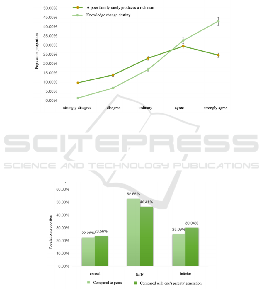
Figure 2: Individuals' views on intergenerational income flows (Photo/Picture credit: Original).

As is shown in Figure 3, more than 75% of the people

surveyed agree with the idea that knowledge can

change their fate, while only 8% disagree with it. It

can be seen that with the development of The Times,

more than enough people have felt the power of

knowledge and the influence on their fate. The

number of people who agree with the view that a poor

family rarely produces a good son is nearly 54%,

more than half, only 23% of the people have a

pessimistic attitude towards the current era, and think

that a person's success is relatively closely related to

their birth.

4.3 The Cognition of One's Income

Figure 3: Individual's own income comparison cognition (Photo/Picture credit: Original).

As can be seen from Figure 4, about half of the

people think that their income is similar to that of their

parents and peers, and about 25% of the people think

that they are above or below the level of their peers.

Currently, 24% of people think their income is higher

than that of their parents' generation, 30% think it is

Research on the Current Situation of Intergenerational Income Flow and Its Inﬂuencing Mechanism

563

lower than that of their parents' generation, and 46%

of people think their income is the same as that of

their parents' generation. Their parents are still the

breadwinner of their families, and they are gradually

bearing the burden of family income. The income of

the whole society is also at a relatively healthy and

stable level.

5 ANALYSIS OF INFLUENCING

FACTORS OF CHILD INCOME

BASED ON MULTIPLE LINEAR

REGRESSION MODEL

Through descriptive statistics, it has a certain

understanding and cognition of the CS of

intergenerational mobility in today's society. In order

to better study the mechanism of intergenerational

income mobility, it first analyzes the influencing

factors of children's income, and select a OLS model

to carry out multiple linear regression of children's

income.

5.1 Model Selection

In the regression prediction of child income, the

logarithm of child income is selected as the dependent

variable, and the dependent variable is calculated by

logarithmic processing of Q8, which is the

quantitative data. Therefore, the multiple linear

regression model is selected to analyze various

factors affecting the child income.

5.2 Variable Setting

In this model construction, six indicators such as

"personal basic information", "parents' basic

information", "education concept", "CS view",

"income comparison" and "family help" are selected

for measurement, and 21 characteristics, including

age, gender, and educational background, are broken

down into these six indications, which are set as

as independent variables that may

affect children's income.

5.3 Model Construction

When multiple linear regression is carried out, the

complete multicollinearity problem of the data will be

detected automatically, and the output results are

shown in Table 8.

Table 8:

OLS regression results

Variables Child income pair value

Father's income pair

value

0.25

***

(0.018)

Maternal income pair

value

0.15

(0.013)

Children's years of

schooling

0.031

***

(0.010)

Sex

-0.139

***

(0.021)

Age

0.191

***

(0.048)

Whether reading

0.468

***

(0.085)

Health status

0.030

(0.012)

Household registration

status

0.021

(0.032)

Father's years of

education

0.100

(0.013)

Years of schooling for

mothers

0.008

***

(0.016)

Real estate per capita

0.229

***

(0.040)

Human capital input

0.394

***

(0.056)

The degree to which

families value education

0.239

***

(0.047)

Perceptions of

intergenerational mobility

0.143

(0.197)

Perceptions of one's own

income

0.179

(0.211)

Degree of subjective

perception of family help

0.012 *

(0.114)

Constant term

4.093

***

(0.693)

Observed value 849

0.798

Note: "***", "**", and "*" indicate significant at 1%, 5%,

and 10% significance levels, respectively; () inside is

clustering standard error.

IAMPA 2025 - The International Conference on Innovations in Applied Mathematics, Physics, and Astronomy

564

5.4 Model Test

For regression models, the homoscedasticity

hypothesis

which

is considered to occur if it occurs that the

variance

of the random error term is no longer constant for

different sample points. In the significance test of a

variable, the

statistic:

()

221

ˆˆ

(0,1,2,,)

()

jj jj jjj

uujj

tjk

cXX

ββ ββ β β

σσ

−

−− −

=== =

(2)

Contains the common

variance of the random

error terms. If heteroscedasticity is present and the

statistic is still calculated according to the formula

used in the case of homoscedasticity, the

statistic

will be distorted, thus invalidating the

test. In short,

heteroscedasticity affects whether the inference is

valid and will reduce the efficiency of the estimation,

so it tests the heteroscedasticity of the regression

model.

The difference between the two can be used to

quantify conditional heteroscedasticity because under

conditional homoscedasticity, the robust standard

error is reduced to the common standard error.

Examining if the robust standard error and the

ordinary standard error are comparable is the informal

approach. This concept is the foundation of the White

test, which White first presented in 1980.

White test has the advantage of testing any form

of heteroscedasticity and is widely applicable.

Therefore, White test is carried out on the established

multiple linear regression model, and the output is as

follows:

The null hypothesis is that the disturbance term does

not exist heteroscedasticity, because the

value is

greater than 0.05, so the null hypothesis is not

rejected, there is no evidence that the disturbance

term exists heteroscedasticity, that is, it is considered

that there is no heteroscedasticity.

Multicollinearity diagnosis can be based on the

Variance Inflation Factor (VIF). A common guideline

is that if VIF>0, the regression equation is considered

to have severe multicollinearity. By using Stata or

other econometric software, if the results show

VIF<0, it generally concludes that the model does not

exhibit serious multicollinearity.

5.5 Analysis of Results

The model's independent variables all pass the

significance test, suggesting that each of them

influences the dependent variable. Meanwhile, when

the regression coefficient of the independent

variable is greater than 0, it indicates that it has a

positive effect on the dependent variable, and vice

versa. According to the obtained

regression

results, the following conclusions can be drawn:

In contrast to the distribution of intergenerational

income elasticity between 0.3 and 0.5 in earlier

studies, the estimated results of the parental income

pair value and the individual income pair value are

significantly positive at the 1% level, with

intergenerational income elasticity values of 0.15 and

0.25, respectively. The possible reasons are as

follows: The data selected in this paper are all current

data, which may lead to the possibility of downward

bias in the results. Therefore, the intergenerational

income elasticity obtained in this paper is relatively

small.

The regression coefficient of gender on individual

income is significantly negative, indicating that

women are in a relatively weaker position than men

in the labor market, and therefore may be in a lower

income level than men. This is consistent with the

reality, which is also one of the urgent problems to be

solved.

Personal income rises with age and with

increasing academic degrees, according to the

regression results of age and years of schooling,

which are statistically positive at the 1% significance

level. Family education and support are crucial for the

rise of personal income, as seen by the significantly

positive regression results of family emphasis on

education and family assistance to individual income

at the significant levels of 1% and 10%, respectively.

The regression coefficients of personal income on

health, education, and per capita household property

are significantly positive. The reasons may be as

follows: First, having a healthy body can more

effectively exert the value created by the body in the

work, and thus obtain higher personal income. At the

same time, parents can reduce the expenditure on

medical care for their children, to reduce the degree

of dependence of children on their parents; Secondly,

in the case of non-schooling, individuals can replace

more valuable work experience and income through

the opportunity cost of non-schooling, to reduce their

dependence on parents.

Research on the Current Situation of Intergenerational Income Flow and Its Inﬂuencing Mechanism

565

6 CONCLUSION

The data analysis of the comprehensive questionnaire

survey shows that there are discussions about

intergenerational mobility on the Internet, and most

of them hold a positive attitude towards future

development after rational thinking about the social

status quo. At the same time, the help provided by

parents in the growth, education and employment of

their children cannot be ignored. To better study the

mechanism of intergenerational income flow, the

research team first conducted a regression analysis on

the influencing factors of child income, and found

that parental income, gender, age, years of education,

health level, whether they are studying or not, and real

estate per capita of the family have significant effects

on child income.

Regression analysis shows that among education

parameters, the number of years of education has a

substantial positive effect on children's income.

Applying the model of intergenerational income, it is

necessary to strengthen the investment of public

education resources, especially public education

resources. And promote the dynamic balance of high-

quality education resources, so as to improve the level

of intergenerational income mobility of the whole

society.

From the above analysis, we have reason to

believe that higher education needs to further

strengthen the adaptation to the market, that is, to

explore the market demand with The Times. For

example, strengthen technical training and practical

courses, to improve the quality of technical ability.

According to the results of the moderated

mediation model, the intergenerational income

elasticity of families with good educational ideas is

lower. Adhere to the good family education concept,

cultivate more excellent children. "Strict" as the first,

seize the children's learning critical period; Cultivate

independent consciousness, so that children do not

have dependent thoughts; Pay attention to children's

growth, communicate with them more, guide children

correctly; Home and school contact, maintain

consistency, support together.

REFERENCES

Becker, G.S. and Tomes, N. (1979). An Equilibrium Theory

of the Distribution of Income and Intergenerational

Mobility. The Journal of Political Pa, 87(6), 1153-1189.

Solon, G. (1992). Intergenerational Income Mobility in the

United States. American Economic Review, 82(3), 393-

408.

Bjorklund, A. and Jantti, M. (1997). Intergenerational

Income Mobility in Sweden Compared to the United

States. American Economic Review, 87(5), 1009-1018.

Haider, S.J. and Solon, G. (2006). Life-Cycle Variation in

the Association between Current and Lifetime Earnings.

American Economic Review, 96(6), 1308-1320.

Dahl, M.W. and De Leire, T. (2008). The Association

Between Children's Earnings and Fathers' Lifetime

Earnings: Estimates Using Administrative Data.

University of Wisconsin-Madison, Institute for

Research on Poverty.

Chernozhukov, V. and Hansen, C. (2007). Instrumental

Variable Quantile Regression: A Robust Inference

Approach. Journal of Econometrics, 142(1), 379-398.

Zhang, M. (2024). Research on Blocking Intergenerational

Transmission of Relative Poverty in Rural Families

Through Education. Huazhong Agricultural University.

Wang, S. (2023). Education Research on the Influence of

Intergenerational Income Mobility in China. Henan

Finance and Economics University of Political Science

and Law.

Levi, G.G., Limor, G. and A.M.S. (2018). Intergenerational

Mobility and the Effects of Parental Education, Time

Investment, and Income on Children’s Educational

Attainment. Review, 100(3).

Chen, C. (2023). Precise Poverty Alleviation and

Intergenerational Mobility in China. Taylor and Francis.

Shu, W., Xiao, Y., Kuo, Z. et al. (2022). How Does

Education Affect Intergenerational Income Mobility in

Chinese Society? Review of Development Economics,

26(2), 774-792.

IAMPA 2025 - The International Conference on Innovations in Applied Mathematics, Physics, and Astronomy

566