ARIMA vs. Machine Learning in Portfolio Return Forecasting: A

Comparative Study Integrating GARCH-Based Volatility Estimation

and Value-at-Risk Applications

Ruiheng Chen

College of International Management (APM), Ritsumeikan Asia Pacific University, Beppu, Oita 874-0011, Japan

Keywords: Time Series, Machine Learning, Value-At Risk.

Abstract: This study aims to compare the application effects of traditional econometric models and machine learning

models in portfolio return prediction and risk management, and selects Apple's daily return as sample data.

First, the Augmented Dickey-Fuller test is used to confirm the data stationarity. The optimal ARIMA model

is constructed under the AIC and BIC criteria, and its in-sample return is predicted. In order to further

characterize the return volatility characteristics, ARCH-LM test and residual square ACF analysis are

performed on the ARIMA model residuals, and then the GARCH model is established to obtain the in-sample

volatility forecast. Based on this, an LSTM model with 25-order lag as input is constructed, and the model is

trained using the full sample data to generate the in-sample forecast of the return. Finally, under the premise

of controlling the confidence level to 95% and uniformly using the GARCH volatility forecast results, the

Value at Risk (VaR) is calculated using the normal distribution assumption, and the VaR of the ARIMA,

LSTM models and real return data are compared and analysed. The research results show that the LSTM

model is more sensitive to the ARIMA model under extreme market volatility conditions, but both have the

limitation of underestimating extreme risks, which provides a direction for the introduction of methods such

as heavy-tailed distribution or extreme value theory in the future.

1 INTRODUCTION

As the continuous development of the global financial

market and the increasing complexity of financial

assets, portfolio management and risk control have

become key concerns for financial institutions and

investors. Traditional time series methods, such as

econometric models represented by Autoregressive

Integrated Moving Average (ARIMA) model are

widely used in forecasting portfolio returns due to

their advantage in capturing linear dependencies.

However, ARIMA model may only be applicable

to specific seasonal patterns and its utility in long-

term decision making and forecasting is limited

(Shumway and Stoffer, 2016; Devi and Alli, 2013).

On the other hand, in recent years, with the

continuous advancement of machine learning

technologies, models such as Long Short-Term

Memory (LSTM) and random forests have been

widely applied to financial time series analysis (Ho et

https://orcid.org/0009-0008-7332-0271

al., 1997). These models demonstrate significant

advantages in capturing the nonlinear structures in

data and complex interactions among variables,

providing a new technical approach for forecasting

portfolio returns (Feng et al., 2018). In particular,

LSTM model can learn from the time dependencies

in the environment and, without explicitly employing

activation functions within its components, each

LSTM unit is capable of collecting information over

long or short time spans (Girsang et al., 2020).

However, despite the power of deep learning, it

requires substantial data and computational

resources, making ARIMA model potentially more

efficient for small-scale problems (Kontopoulou et

al., 2023). Bollerslev emphasized that in terms of risk

measurement, traditional time series and econometric

models are based on the assumption of constant

variance (Bollerslev, 1986). In contrast, the volatility

characteristics of actual financial markets make

simple mean forecasts inadequate for fully reflecting

risk levels. The Generalized Autoregressive

Chen, R.

ARIMA vs. Machine Learning in Portfolio Return Forecasting: A Comparative Study Integrating GARCH-Based Volatility Estimation and Value-at-Risk Applications.

DOI: 10.5220/0013827000004708

Paper published under CC license (CC BY-NC-ND 4.0)

In Proceedings of the 2nd International Conference on Innovations in Applied Mathematics, Physics, and Astronomy (IAMPA 2025), pages 419-428

ISBN: 978-989-758-774-0

419

Conditional Heteroskedasticity (GARCH) model, as

a classical tool for modeling market volatility, can

effectively characterize these time-varying risk

features (Engle and Patton, 2001).

In addition, Value at Risk (VaR) is an important

tool for risk management and provides a standardized

risk measurement framework, but it needs to be

combined with other methods to fully assess risks

(Duffie and Pan, 1997). Moreover, Alexander and

Baptista illustrated that the minimum VaR portfolio

only exists when the confidence level is high enough,

while a low confidence level will lead to irrational

decisions and market imbalance (Alexander and

Baptista, 2002). In extreme risk scenarios, flexible

GARCH models combined with leptokurtic

distributions can significantly improve the accuracy

of VaR predictions. Therefore, by integrating return

forecasting with GARCH volatility modelling, the

VaR calculation can reflect a stronger sensitivity to

risk and enhanced practical applicability.

Current research has been limited to either

comparing the predictive performance of ARIMA

models with machine learning models or focusing

solely on VaR calculation and forecasting using

GARCH models. Although these studies provide

valuable insights into individual model performance,

there is a clear lack of research that integrates all three

modeling approaches into a cohesive framework for

application in real investment portfolios. This

disjointed approach leaves a gap in understanding

how these models can complement each other in

practical, risk-sensitive forecasting environments.

Based on this background, the present study aims

to bridge this gap by conducting a comprehensive

comparison of ARIMA models and typical machine

learning methods in forecasting portfolio returns. The

research will then incorporate GARCH models for

volatility modeling, leveraging the strengths of each

approach to achieve an accurate estimation of

portfolio VaR. In this integrated framework,

comparing the ARIMA model's capacity to capture

linear trends and seasonality with the machine

learning methods' ability to uncover complex

nonlinear patterns, can provide a more robust and

nuanced forecast of returns. Meanwhile, the GARCH

model's proven track record in modelling volatility

clustering in financial time series will be instrumental

in refining the risk measurement process.

This study can provide a deeper understanding of

the adaptability and limitations of these different

models in real-world forecasting scenarios. By

systematically integrating these models, the research

aims to offer both theoretical and quantitative support

for asset allocation and risk control. The findings are

expected to contribute to the development of more

sophisticated risk management tools that can be

applied by financial institutions and portfolio

managers, enhancing decision-making processes in

environments characterized by uncertainty and

market volatility.

2 METHODOLOGY

In this part, the data resources used in this study,

variables involved and specific methods will be

introduced.

2.1 Data Source

The data utilized in this study is sourced from the

Yahoo Finance platform, an international financial

information platform. The database is accessed and

extracted through Python programming language.

The daily stock data set extracted from the Yahoo

Finance platform contains important indicators such

as opening price, closing price, and returns, which can

clearly reflect the daily changes of the stock. To

verify the performance of the ARIMA model and

LSTM model in portfolio returns prediction and risk

measurement, this study selected the historical stock

price data of Apple Inc. (stock code: AAPL) as the

research object, with a time span of January 1, 2015

to February 28, 2025, covering significant market

stages such as Covid-19 and the Russian-Ukrainian

War. As a world-renowned technology company,

Apple's stock has high market liquidity and

representativeness, which can better reflect the

dynamic characteristics of market risk and return.

2.2 Variables Selection and Description

In this study, the daily returns extracted from the

stock data were selected as the basic indicator,

comprising approximately 2,553 observations.

Subsequent data processing on this variable yielded

three additional variables. Ultimately, these variables

were utilized to compute the VaR using two different

prediction models and GARCH model, leading to the

corresponding risk estimates.

2.3 Method Interpretation

In this study, Augmented Dickey-Fuller (ADF) test

was first conducted on the extracted daily returns of

Apple Inc. to examine the presence of unit roots

within the time series. Upon confirming the

stationarity of the daily returns, an optimal ARIMA

IAMPA 2025 - The International Conference on Innovations in Applied Mathematics, Physics, and Astronomy

420

model was constructed based on the Akaike

Information Criterion (AIC) and the Bayesian

Information Criterion (BIC), and in-sample forecasts

were generated to obtain the corresponding expected

return predictions.

𝛻



𝑥



=𝑐+

∑

𝜙







𝛻



𝑥



∑

𝜃







𝜖



(1)

where 𝛻



𝑥



is the value of the time series 𝑥



after d

differences, 𝑐 is the constant term, 𝑝 represents the

order of the autoregressive component, 𝜙



denotes

the autoregressive coefficients, and 𝛻



𝑥



indicates

the lagged value at period 𝑖 of the differenced series,

𝑞 represents the order of the moving average

component, 𝜃



denotes the moving average

coefficients, and 𝜖



indicates the lagged value at

period i of the error term (Kontopoulou et al., 2023).

Building on the optimal ARIMA model, the

ARCH-LM test on its residuals was conducted to

assess the presence of ARCH effects. In addition, the

ACF of the squared residuals was plotted to further

examine the significance of these effects. Following

this, a GARCH (1,1) model was established, and in

sample forecasts were conducted to derive volatility

predictions.

𝜎





=𝑎



∑

𝑎







𝜖





∑

𝑏







𝜎





(2)

where

∑

𝑎







∑

𝑏







<1.

Additionally, a machine learning approach was

employed by constructing an LSTM model with a lag

order of 25. This model was trained using the full

sample of data, and in-sample forecasts were

produced to generate expected return predictions.

For the final stage of the analysis, VaR estimates

were computed under normal distribution. To ensure

a fair comparison of the portfolio VaR performance

between the ARIMA model and the LSTM model, a

set of control variables was maintained, including the

adoption of a unified confidence level of 95%, and the

use of volatility forecasts derived from the GARCH

model. The results were then visualized for

comparative observation.

𝑉𝑎𝑅 = −𝜇 + 𝑧



𝜎 (3)

where 𝜇 represents the returns, 𝜎 denotes the

standard deviation of returns, and 𝑧



is the quantile of

the standard normal distribution corresponding to the

confidence level p.

3 RESULTS AND DISCUSSION

This section will elaborate on the process and final

results of the ARIMA model, GARCH model and

LSTM model used in this study in data processing,

model construction and forecasting analysis. In

addition, the prediction effects of the ARIMA model

and the LSTM model are further compared in a

quantitative manner through the VaR calculation

results. Table 1 presents the dataset of daily returns

from 2015-01-05 to 2025-02-27 of Apple Inc.

Table 1: Apple Inc. Daily Returns.

Date Return

2015-01-05 -0.028

2015-01-06 0.000

2015-01-07 0.014

2015-01-08 0.038

2015-01-09 0.001

……

2025-02-21 -0.001

2025-02-24 0.006

2025-02-25 -0.000

2025-02-26 -0.027

2025-02-27 -0.013

3.1 ARIMA Model Consequence

The figure 1 is a time series plot of the rate of return

over time. The result of the ADF test on the sample

time series data is that the test value (ADF Statistic)

is -15.806, and the p-value is close to 0.00, indicating

that the null hypothesis of "the existence of a unit root

in the time series dataset" can be rejected at an

extremely low significance level, which means the

time series is statistically stationary and does not

require further differential processing to meet the

requirements of subsequent modelling.

ARIMA vs. Machine Learning in Portfolio Return Forecasting: A Comparative Study Integrating GARCH-Based Volatility Estimation and

Value-at-Risk Applications

421

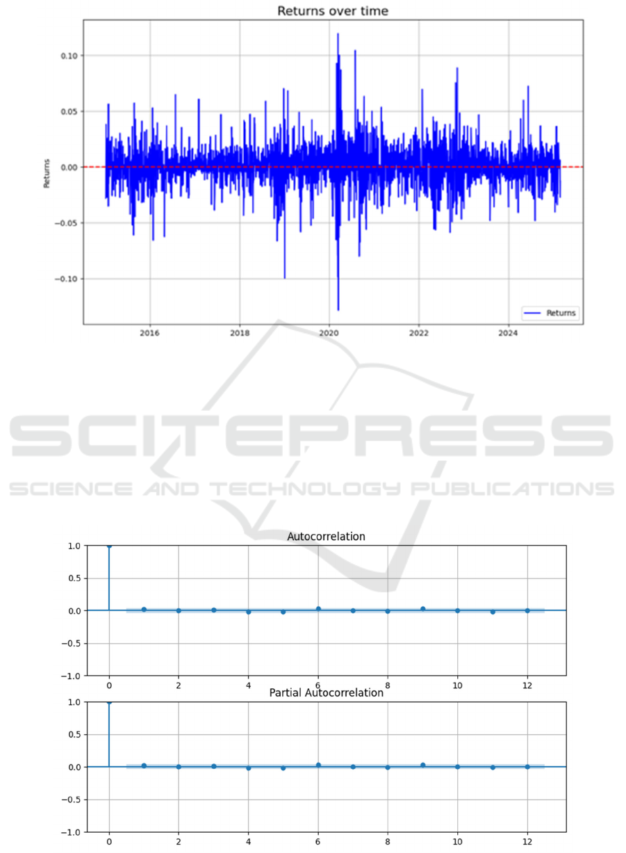
Figure 1: Apple Inc. Daily Return Time Series Plot 2015-01-05 to 2025-02-27 (Picture credit: Original)

According to the ACF and PACF plots of the

residuals of the ARIMA models based on the AIC and

BIC criterion presented in Figure 2 and Figure 3, it

can be found that the residuals of the two optimal

models, the ARIMA(3, 0, 5) by AIC and the

ARIMA(0, 0, 1) by BIC, lie within the range of the

confidence intervals for each lag period, with no sign

of significant deviation from the zero axis. This

indicates that the residuals of both models exhibit

stochastic characteristics close to white noise,

suggesting that the models fit the linear structure of

the data more adequately. However, considering the

model complexity and the number of parameters, the

ARIMA(0,0,1) model chosen by the BIC is more

concise and more practical, and therefore the

ARIMA(0,0,1) model of the BIC is taken as the final

optimal model.

Figure 2: ACF and PACF Plots of ARIMA Model Residuals Based on AIC Criteria (Picture credit: Original)

IAMPA 2025 - The International Conference on Innovations in Applied Mathematics, Physics, and Astronomy

422

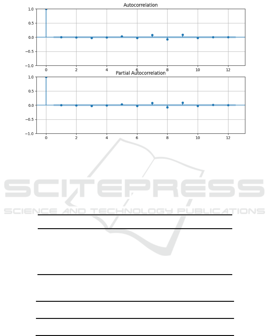
Figure 3: ACF and PACF Plots of ARIMA Model Residuals Based on BIC Criteria (Picture credit: Original)

The established optimal ARIMA model was tested for

fitness and the SARIMAX results are shown in Table

2 and Table 3. According to the results, both the

constant term, const=0.0011, and the MA(1) term,

ma.L1=-0.0663, are significant, indicating that the

studied return series is characterized by a significant

level of average daily returns and short-term negative

autocorrelation. In addition, the Ljung-Box test of the

model residuals, Prob(Q)=0.99, shows that there is no

significant autocorrelation in the residuals, indicating

that the model has effectively captured the linear

autocorrelation structure of the dataset.

Table 2: ARIMA(0, 0, 1) SARIMAX Results (1)

coef std err z P>|z| [0.025 0.975]

const 0.0011 0.000 3.162 0.002 0.000 0.002

ma.L1 -0.0663 0.013 -5.172 0.000 -0.091 -0.041

stigma2 0.0003 0.000 62.401 0.000 0.000 0.000

Table 3: ARIMA(0, 0, 1) SARIMAX Results (2)

Ljung-Box (L1) (Q) 0.00 Heteroskedasticity (H) 1.33

Prob (Q) 0.99 Prob (H) (two-sided) 0.00

Finally, the established model is utilized to perform

in-sample prediction on the dataset. The results are

shown in Table 4.

As can be observed from the figure 4, the actual

returns (blue line) are significantly more volatile and

exhibit significant volatility aggregation.

ARIMA vs. Machine Learning in Portfolio Return Forecasting: A Comparative Study Integrating GARCH-Based Volatility Estimation and

Value-at-Risk Applications

423

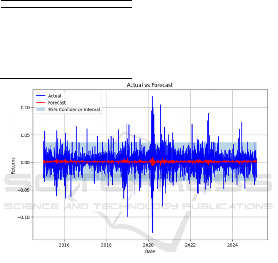
Table 4: ARIMA Model Returns Prediction Results

Date Return ARIMA

2015-01-05 0.020028

2015-01-06 0.020421

2015-01-07 0.019741

2015-01-08 0.019295

2015-01-09 0.020509

… …

2025-02-21 0.015236

2025-02-24 0.014822

2025-02-25 0.014470

2025-02-26 0.014094

2025-02-27 0.015101

In contrast, the overall volatility of the returns

predicted by the ARIMA model (red line) is small and

close to zero, indicating that the model lacks the

ability to effectively capture extreme volatility in

financial market returns. In addition, the 95%

confidence intervals (light blue area), while covering

most of the actual return data points to a certain extent,

are too conservative in the vicinity of extremes, such

as the sharp fluctuations in the early 2020s (Covid-19

time shock), and do not fully reflect the true level of

risk in the market.

Figure 4: ARIMA Model Forecast vs. Actual Returns (Picture credit: Original)

3.2 GARCH (1,1) Model Consequence

According to the results shown in Table 3, the

heteroscedasticity test (Prob(H)=0.00) also indicates

the presence of significant conditional

heteroscedastic effects in the residuals. To ensure the

effective establishment of a GARCH model, an

ARCH-LM test was conducted on the residuals of the

ARIMA(0,0,1) model. The ARCH-LM test p-value is

0. Besides, from the squared residuals ACF plot, it is

clear to observe that for many lag orders, the

correlation coefficients remain outside the range

under the null hypothesis of no autocorrelation-

particularly pronounced in the first few lags. These

results indicate that the ARIMA(0,0,1) model has not

fully captured the volatility of the return series, and

significant ARCH effects persist in its residuals.

Therefore, the GARCH (1,1) model was constructed

and the in-sample volatility prediction is shown in

Table 5.

IAMPA 2025 - The International Conference on Innovations in Applied Mathematics, Physics, and Astronomy

424

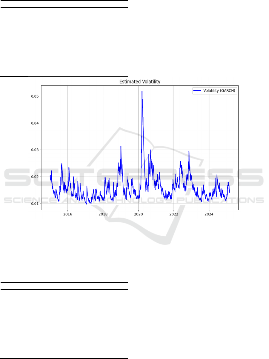
Table 5: GARCH (1,1) Model Prediction Results

Date Volatilit

GARCH

2015-01-05 0.020

2015-01-06 0.020

2015-01-07 0.020

2015-01-08 0.019

2015-01-09 0.021

… …

2025-02-21 0.015

2025-02-24 0.015

2025-02-25 0.014

2025-02-26 0.014

2025-02-27 0.015

The variation of in-sample volatility prediction

demonstrated in figure 5 indicates that the volatility

estimated by the GARCH (1,1) model shows

significant time-varying characteristics throughout

the sample period, and exhibits an obvious "volatility

clustering" phenomenon: when there are large shocks

or major events in the market, such as the extreme

market conditions in early 2020, the volatility will

rise significantly, even reaching above 0.05, while in

relatively stable market periods, it will remain at a

low level, approximately in the range of 0.01 to 0.02.

Figure 5: GARCH (1,1) Model In-Sample Volatility Prediction (Picture credit: Original)

3.3 LSTM Model Consequence

The LSTM model in-sample prediction result is

shown in Table 6.

Table 6: LSTM Model Returns Prediction Results

Date Return LSTM

2015-02-10 0.001

2015-02-11 0.001

2015-02-12 0.001

2015-02-13 0.001

2015-02-17 0.001

… …

2025-02-21 0.000

2025-02-24 -0.000

2025-02-25 0.000

2025-02-26 -0.000

2025-02-27 -0.000

According to the prediction results depicted in Figure

6, it is clear to see the LSTM model’s in-sample

predictions for returns generally align with the actual

returns (blue line) in terms of overall trends. However,

during periods of significant market fluctuations or

extreme events, such as the Covid-19 outbreak in

early 2020, the model’s predictions (red line) fall

short of capturing the substantial swings in actual

returns, leading to some degree of underestimation or

overestimation. Overall, while the LSTM model

demonstrates feasibility in capturing routine volatility

and trends, it still shows certain limitations in

handling abnormal shocks and extreme market

conditions.

ARIMA vs. Machine Learning in Portfolio Return Forecasting: A Comparative Study Integrating GARCH-Based Volatility Estimation and

Value-at-Risk Applications

425

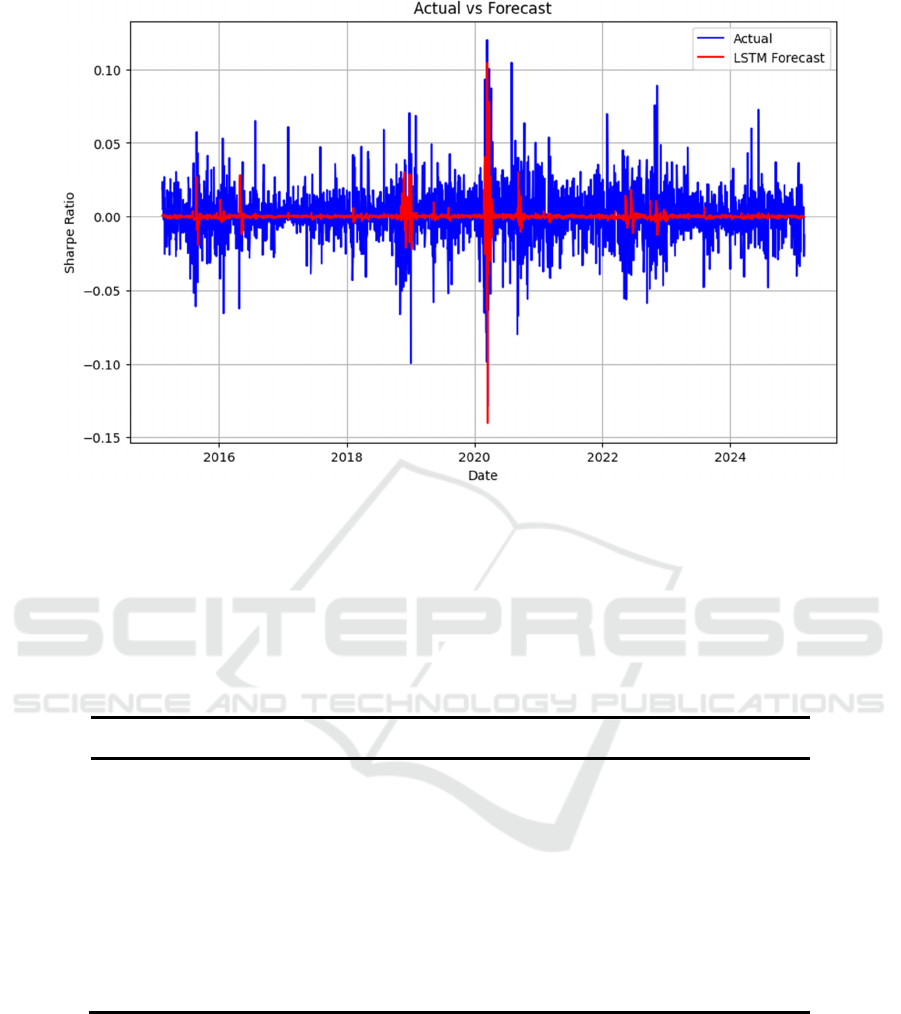
Figure 6: LSTM Model Forecast vs. Actual Returns (Picture credit: Original)

3.4 LSTM Model Consequence

The VaR of the portfolio is calculated based on the

in-sample data and all the collected forecast data, and

the results are shown in Table 7.

Table 7: Calculated VaR Results

Date Var-In Sample VaR-ARIMA VaR-LSTM

2015-02-10 0.010 0.029 0.029

2015-02-11 0.006 0.030 0.028

2015-02-12 0.017 0.030 0.029

2015-02-13 0.024 0.029 0.029

2015-02-17 0.023 0.028 0.028

... ... ... ...

2025-02-21 0.026 0.024 0.025

2025-02-24 0.018 0.023 0.025

2025-02-25 0.024 0.023 0.023

2025-02-26 0.050 0.022 0.023

2025-02-27 0.038 0.022 0.025

According to the VaR variation trend in Figure 7, it

can be seen that the VaR calculated based on real

returns (light pink curve) showed large fluctuations

during the sample period, especially reaching a peak

in the extreme market environment in early 2020,

reflecting the huge risks faced by the market. In

contrast, the VaR obtained by the ARIMA model

(blue line) is relatively stable overall. Although it can

remain stable during regular volatility periods, it

appears to be insufficiently responsive when facing

extreme market events and fails to fully capture the

increase in extreme risk exposure. The LSTM model

(red line) is between the two. Its VaR estimate is not

much different from ARIMA in normal situations, but

it shows higher and sharper jumps when facing more

drastic volatility environments, indicating that it has

a more sensitive response to sudden fluctuations to a

certain extent.

IAMPA 2025 - The International Conference on Innovations in Applied Mathematics, Physics, and Astronomy

426

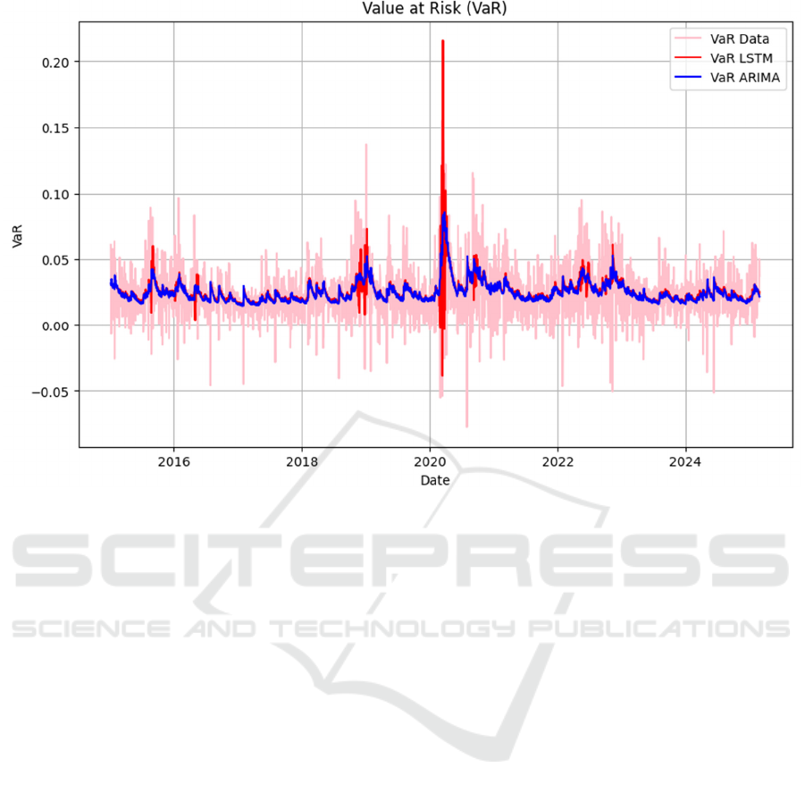
Figure 7: Calculated VaR Results Comparison (Picture credit: Original)

4 CONCLUSION

In conclusion, based on the result of the VaR

estimation performance of the ARIMA and LSTM

models, it can be concluded that the LSTM model

demonstrates greater sensitivity to extreme market

volatility, offering a relatively superior capability in

capturing tail risks compared to ARIMA.

However, this study is still subject to certain

limitations. The VaR calculation employed in this

research relies on the assumption of normal

distribution, which may not adequately represent the

skewness and fat-tail characteristics commonly

observed in financial markets, potentially resulting in

underestimation of tail risks during extreme market

conditions. Besides, the models utilized only a single

dataset, ignoring the impact of multi-dimensional

information on risk such as macroeconomic

indicators, industry information, and market

sentiment. In addition, the LSTM model has a high

demand for data volume during training and

parameter tuning, and if the data quality or quantity is

insufficient, it also affects the robustness and

generalization ability of the model.

Therefore, in future research, the models can

integrate with more flexible methods such as heavy-

tailed distributions into the VaR estimation

framework to more accurately reflect tail risk in

extreme market environments. Additionally, for the

dataset, it is possible to further integrate multi-source

data, such as macroeconomic indicators, company

financial data, news public opinion and social media

sentiment, etc., which are heterogeneous information.

This will provide the model with richer risk signals,

with the aim of improving the accuracy and

robustness of the prediction. Moreover, the study can

be extended to a wider range of risk measures,

including Expected Shortfall, Max Drawdown, etc.,

or to explore how model uncertainty measures can be

combined for more comprehensive risk management,

helping regulators and investment managers better

understand and utilize risk predictions from model

outputs.

REFERENCES

Alexander, G. J., Baptista, A. M., 2002. Economic

implications of using a Mean-VAR model for portfolio

selection: A comparison with Mean-Variance analysis.

SSRN Electronic Journal.

Bollerslev, T., 1986. Generalized autoregressive

conditional heteroskedasticity. Journal of

Econometrics, 31(3), 307-327.

ARIMA vs. Machine Learning in Portfolio Return Forecasting: A Comparative Study Integrating GARCH-Based Volatility Estimation and

Value-at-Risk Applications

427

Devi, B., Alli, P., 2013. An effective time series analysis

for stock trend prediction using ARIMA model for

Nifty Midcap-50. International Journal of Data Mining

& Knowledge Management Process, 3(1), 65-78.

Duffie, D., Pan, J. 1997. An overview of value at risk. The

Journal of Derivatives, 4(3), 7-49.

Engle, R. F., Patton, A. J., 2001. What good is a volatility

model? Quantitative Finance, 1, 237-245.

Feng, G., He, J., Polson, N. G. 2018. Deep learning for

predicting asset returns. Papers.

Girsang, A. S., Lioexander, F., Tanjung, D. 2020. Stock

price prediction using LSTM and search economics

optimization. International journal of computer

science.

Ho, S., et al. 1997. Long short-term memory. Neural

Computation, 9(8), 1735-1780.

Kontopoulou, V. I., Panagopoulos, A. D., Kakkos, I.,

Matsopoulos, G. K., 2023. A Review of ARIMA vs.

Machine Learning Approaches for Time Series

Forecasting in Data Driven Networks. Future Internet,

15(8), 255.

Shumway, R. H., Stoffer, D. S., 2016. Time Series Analysis

and its applications. Journal of Econometrics.

IAMPA 2025 - The International Conference on Innovations in Applied Mathematics, Physics, and Astronomy

428