Enhancing Resilience of Strong Structural Controllability in

Leader-Follower Networks

Vincent Schmidtke

and Olaf Stursberg

Control and System Theory, EECS Dept., University of Kassel, Germany

Keywords:

Strong Structural Controllability, Leader-Follower Networks, Edge Augmentation, Resilient Control.

Abstract:

This paper explores measures of edge augmentation to enhance resilience of strong structural controllability

for control systems modeled as leader-follower networks. Unlike existing methods which typically increase the

number of leaders, the proposed approach achieves resilience by strategically adding edges, thus maintaining

leader sets with a small cardinality. Using the zero forcing method, conditions are derived to enhance resilience

either for speciﬁc agents or for the entire network. Numeric simulations validate the approach and show its

effectiveness in large and complex networks.

1 INTRODUCTION

Networked Control Systems (NCS) are integral to

modern engineering, enabling distributed coordina-

tion and scalability in complex systems such as smart

grids, trafﬁc systems, swarms and biological net-

works. In these systems, it is frequently desired to

control the network by injecting control actions only

for a small subset of nodes. This leads to the notion

of leader-follower frameworks, where leaders have a

control input, whereas followers do not have one (Por-

ﬁri and di Bernardo, 2008; Egerstedt et al., 2012).

While this can simplify the control architecture, the

system may get more fragile with respect to malfunc-

tions or attacks, if the loss of an agent and/or its con-

nections signiﬁcantly impairs the system’s function-

ality (Pasqualetti et al., 2020).

Controllability and resilience are thus important

properties when investigating in how far such systems

can maintain their function if subject to internal or

externally triggered changes. Controllability ensures

the ability to let the system transition from any ini-

tial state to a desired state, while resilience pertains to

the system’s capacity to withstand (or recover from)

disruptions. These properties are crucial, especially

in safety-critical applications where failures can have

catastrophic consequences.

This paper focuses on the notion of strong struc-

tural controllability (SSC) which requires controlla-

bility for varying interconnections of states (and thus

structures) of the system to be controlled. This is par-

https://orcid.org/0009-0006-6322-103X

https://orcid.org/0000-0002-9600-457X

ticularly advantageous in NCS, since controllability

depends on the network topology and the leader set,

rather than only particular weights assigned to con-

stantly existing interconnections. This makes SSC

suitable for real-world applications, in which infor-

mation on edge weights may be uncertain, time-

varying, noisy, or even vanishing (Chapman and Mes-

bahi, 2013; Monshizadeh et al., 2014).

In order to assess SSC of leader-follower networks

as well as its resilience against changing network

topologies, this paper utilizes the method of zero forc-

ing sets, a graph-theoretic approach that is frequently

used in the context of SSC for NCSs (Monshizadeh

et al., 2014; Abbas et al., 2020b; Schmidtke et al.,

2024). In the context of SSC, the following exist-

ing papers have proposed edge augmentation, i.e. the

addition of edges to a graph, as a means to modify

the system structure for enhanced controllability. In

(Chen et al., 2019), minimal edge sets are computed

to render non-SSC systems structurally controllable,

whereas (Abbas et al., 2020a) and (Mousavi et al.,

2021) identify a set of edges that can be added without

violating SSC. These approaches leverage edge aug-

mentation as a design tool to either restore or preserve

controllability.

A certain body of literature in the given con-

text has examined the relationship between graph-

theoretic robustness measures and the minimum num-

ber of required leaders: The most often used mea-

sure is the Kirchoff index, which formulates the sys-

tem’s resilience against disconnection. (Pasqualetti

et al., 2020) and (Abbas et al., 2020b) investigate the

trade-off between an increasing connectivity and the

minimum number of required leader agents, which is

136

Schmidtke, V. and Stursberg, O.

Enhancing Resilience of Strong Structural Controllability in Leader-Follower Networks.

DOI: 10.5220/0013826200003982

Paper published under CC license (CC BY-NC-ND 4.0)

In Proceedings of the 22nd International Conference on Informatics in Control, Automation and Robotics (ICINCO 2025) - Volume 1, pages 136-144

ISBN: 978-989-758-770-2; ISSN: 2184-2809

also discussed as a central controllability measure in

(Egerstedt et al., 2012). The work in (Abbas et al.,

2024) identiﬁes edge additions leading to a reduction

of the required number of leader agents, while in-

creasing the robustness measure. A design procedure

which builds a graph which is SSC with the highest

possible Kirchoff index for speciﬁed graph parame-

ters is presented in (Patel et al., 2024).

The notion of robustness addressed in the afore-

mentioned work differs from the approach to re-

silience taken in this paper. Rather than focusing

on graph connectivity, resilience of controllability is

here speciﬁcally considered with respect to preserv-

ing SSC in case of structural disruptions such as node

or edge failures. Resilient SSC is addressed only in

very few contributions: In (Schmidtke et al., 2024),

conditions have been speciﬁed which allow to check

which agents can be removed from the system, while

maintaining SSC with the current leader set. The pa-

pers (Abbas, 2023) and (Alameda et al., 2024) exploit

methods to specify a set of leader agents which guar-

antees that a certain number of nodes or edges can be

removed, while keeping the system SSC. However,

these methods require the introduction of far more

leader agents – this, on the one hand, leads to leader

selection problems which are known to be NP-hard in

general (Aazami, 2008). On the other hand, this ap-

proach contradicts the goal to have as few leaders as

possible. Thus overall, a signiﬁcant gap in literature is

the enhancement of resilience without increasing the

number of leader agents. This paper addresses this

gap by proposing schemes to augment the graph by

additional edges in order to achieve strong structural

controllability, including the case that agents leave

and/or join the network.

The paper is structured as follows: Section 2 intro-

duces preliminaries on the system class, the property

of strong structural controllability, and the zero forc-

ing method. Section 3 formally states the problem

of enhancing resilient strong structural controllability

through modifying the edges of the graph. Section 4

presents the main results, while Section 5 provides a

numeric example to illustrate the approach. Finally,

Section 6 concludes the paper, summarizing the ﬁnd-

ings and their implications.

2 PRELIMINARIES

Networks are in this paper represented by a graph

G = (V ,E,W ), in which V = {1,..., N} is the set of

agents, E the set of edges, and W the set of weights

assigned to each edge according to w

i j

: E → R \ 0.

For simpliﬁcation, it is assumed that (i, j) ∈ E ⇔

( j,i) ∈ E, which simpliﬁes the notation. However,

i j

̸= w

is allowed, making the graph directed. It

is important to note, that the upcoming results can

be straightforwardly extended to cases where the as-

sumption of bi-directional edges is dropped. Edges

(i,i) for representing self-loops are permitted. Let all

neighbors of a node i be collected in a set N

= { j ∈

V |( j, i) ∈ E, j ̸= i}.

The set of agents is divided into a set of leader

agents V

= {l

,.. .,l

} ⊆ V and the set of follower

agents V \ V

. The m

leaders have a control input

(t) and the dynamics:

˙x

(t) = w

· x

(t) +

∑

j∈N

i j

· x

(t) + u

(t), (1)

while the dynamics of the followers:

˙x

(t) = w

· x

(t) +

∑

j∈N

i j

· x

(t) (2)

lacks an input. Note that with this deﬁnition the lead-

ers are allowed to interact dynamically with follower

and leader agents. The initial state of any agent is de-

noted by x

(0) = x

i,0

The global dynamics of all agents can be

derived by introducing the state vector x(t) :=

(t),x

(t),. .., x

(t)]

∈ R

, the input vector

u(t) := [u

(t),u

(t),. .., u

]

∈ R

, the weight ma-

trix W with elements w

i j

, and the leader selection ma-

trix B ∈ [0,1]

N×m

according to:

B =

(

i j

= 1 if i = l

0 otherwise.

(3)

The global dynamics of the network can then by writ-

ten as:

˙x(t) = W x(t) + Bu(t), (4)

in which the leader agents can be controlled, whereas

the follower agents only respond to the behavior of

the leader agents.

2.1 Strong Structural Controllability

As is well known, a system (4) is controllable if the

following matrix has full rank (Antsaklis and Michel,

1997):

R(W,B) =



B W B ... W

n−1



, (5)

In networked systems, however, edge weights are of-

ten either unavailable or time-varying, rendering the

direct use of (5) impractical. Then, strong structural

controllability (SSC) becomes relevant, as it assesses

controllability solely based on the system’s structure,

independent of the speciﬁc edge weights. To deﬁne

Enhancing Resilience of Strong Structural Controllability in Leader-Follower Networks

137

SSC, the following family of matrices associated with

a given graph

G is considered:

W (

G) = {W ∈ R

N×N

: for i ̸= j, w

i j

̸= 0 ⇔ ( j,i) ∈ E}.

(6)

This matrix family includes all matrices for which the

nonzero off-diagonal entries correspond exactly to the

edges of

G. Note that the diagonal elements of every

W ∈ W (

G) can be arbitrary. With this notation, SSC

can be deﬁned as follows:

Def. 1 (Strong Structural Controllability). A linear

system according to (4) is SSC if and only if the pair

(W,B) is controllable for all W ∈ W (

G), where B rep-

resents the agents through which inputs are applied.

Aiming at SSC according to this deﬁnition re-

quires that any possible matrix W of the given dimen-

sion needs to be considered, while the zero entries W

are encoded also by the fact that a corresponding edge

is not deﬁned in E. Thus, it is sufﬁcient (without loss

of generality) from here on to refer the considerations

on SSC to a reduced version G = (V ,E) of the graph

G without weights.

2.2 SSC and Zero Forcing

The use of zero forcing as a method to examine SSC

is motivated by its direct correlation to network con-

trollability on graphs, as explained in (Monshizadeh

et al., 2014), see also Theorem 1. Zero forcing is

deﬁned as follows (AIM Minimum Rank - Special

Graphs Work Group, 2008):

Def. 2 (Zero Forcing). For a graph G = (V ,E), let

⊂ V , |V

| > 0 be chosen arbitrarily as an initial

set of colored nodes. Let then V be partitioned into

and a set V

of initially uncolored nodes accord-

ing to V

∩ V

= ∅ and V

∪ V

= V . If a colored

node i then only has one uncolored neighbor j, then j

is forced to be colored by i (denoted by i ⇀ j), i.e. j

is inserted into V

and removed from V

. This color-

ing process continues until no further coloring can be

executed, leading to ﬁnal colored and uncolored sets

and V

ZFC2

ZFC1

1 2

Figure 1: Example for zero forcing with V

as ZFS with

minimal cardinality.

Def. 3 (Derived Set). If zero forcing has started from

and terminated with V

, the latter set is also

called the derived set and is denoted by D(G,V

) :=

Def. 4 (Zero Forcing Set). If a selected set of initially

colored nodes V

leads to D(G, V

) = V (i.e. all

nodes are colored at the end of zero forcing), V

called zero forcing set (ZFS).

In addition the following terms are introduced:

Def. 5 (Forcing Chain). A forcing chain (FC)

C (G, V

) contains the list of forces i ⇀ j obtained

during zero forcing for the graph G, where this list is

sorted according to the sequence of forces carried out

during the forcing procedure when starting from V

Def. 6 (Forcing Agents). For an agent j ∈ V , the

set F

(G,V

) contains all forcing agents (FA) i ∈ V ,

which can color j through a force i ⇀ j contained in

any forcing chain C (G, V

An example that illustrates these quantities can

be found in Fig. 1. As shown there, forcing chains

generally lack uniqueness, while the derived set

D(G,V

) remains unique (AIM Minimum Rank -

Special Graphs Work Group, 2008). For any set of

FA, the inequality |F

(G,V

)| ≤ |N

| is always sat-

isﬁed because only neighbors are capable of color-

ing an agent. When V

constitutes a ZFS, it en-

sures that |F

(G,V

)| ≥ 1 for all j ∈ V

, guarantee-

ing that at least one FC for every uncolored agent ex-

ists. Accordingly, |F

(G,V

, j)| = 0 for all j ∈ V

since these agents are colored initially.

The following theorem from (Monshizadeh et al.,

2014) establishes that zero forcing can determine if

a leader set V

guarantees strong structural controlla-

bility for the system deﬁned by the graph G:

Theorem 1 ((Monshizadeh et al., 2014)). System (4)

with W ∈ W and B deﬁned by the leader set V

is SSC

if and only if V

is a ZFS for G.

2.3 Resilient SSC

In network controllability, resilience refers to the sys-

tem’s ability to remain controllable despite agent mal-

functions or edge failures (Abbas, 2023). In terms of

structural controllability, the concept of a ZFS is ex-

tended to l-leaky forcing sets, deﬁned as follows:

Def. 7 (l-Leaky Forcing Set). The leader set V

is a l−leaky forcing set (l−LFS), if ∀i ∈ V \ V

(G,V

) ≥ l + 1.

Building on the previous deﬁnition, (Abbas, 2023)

demonstrates that an l-LFS provides resilience against

l malfunctions, where a malfunction may involve a

node departure or edge removal. (Note that the case

ICINCO 2025 - 22nd International Conference on Informatics in Control, Automation and Robotics

138

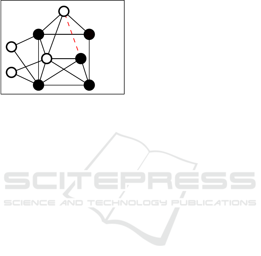
Figure 2: In graph G, node 1 has only node 5 as its only one

forcing agent, i.e., the system is no longer SSC if node 1 is

removed from the graph. In G

′

, which is obtained by adding

the edge indicated by the red dashed line to G, node 5 has

an additional forcing agent, and therefore the graph remains

SSC, if node 1 is removed.

of entering agents is not considered here, but results

on this situation can be found in (Schmidtke et al.,

2024).

3 PROBLEM STATEMENT

While in (Abbas, 2023) the l-LFS guarantees re-

silient SSC by introducing additional leader agents,

the present work aims at improving resilience through

edge augmentation, i.e., by adding new edges to the

graph.

Formally, given a graph G = (V , E) with a ZFS

, the addressed problem is to enhance resilience by

adding an edge (i, j) (where i, j ∈ V and (i, j) ̸∈ E)

such that:

(G,V

)| < |F

′

)|, (7)

for G

′

= (V , E ∪ (i, j)).

This approach, which can be applied iteratively,

follows the principle of the l-LFS methodology by in-

creasing the number of FA for critical nodes. How-

ever, this is achieved through the addition of edges

rather than by expanding the leader set. The method

is particularly well-suited for scenarios in which bot-

tlenecks or vulnerable regions of the network are

known in advance. In such cases, edge augmenta-

tion can be applied in a targeted manner to strengthen

the resilience of speciﬁc nodes, thereby improving

resilience without the need to introduce additional

leader agents.

For instance, in scenarios like the one in Fig. 2,

resilience is ensured by leveraging the result from

(Schmidtke et al., 2024): SSC is preserved, when

an agent j leaves G, provided that for all uncolored

neighbors i ∈ N

the following holds:

(G,V

) \ j| > 0. (8)

To date, no published method systematically explores

possibilities of modifying the set of FA through leader

selection or edge augmentation. Thus, the following

section proposes a framework for strategically mod-

ifying the network topology to enhance resilience of

SSC.

4 IMPROVING RESILIENCE BY

EDGE AUGMENTATION

The primary objective of this section is to establish

conditions that guarantee (at least locally) enhanced

resilience of SSC by augmenting the set E of the

graph G by an additional edge (i, j). To achieve this,

the notion of a forcing graph is introduced. The latter

enables the analysis of the forcing agents of G by

examining how the addition of the edge affects the

network’s resilience. Based on this analysis, a main

theorem is formulated stating conditions under which

the augmentation leads to improved resilience. Fur-

thermore, this section shows that, under the derived

conditions, a ZFS in G retains the SSC properties,

ensuring that resilience is either globally or locally

enhanced.

A forcing graph is introduced to determine which

nodes are colored before a speciﬁc uncolored node,

under the condition that a designated colored node

does not color any other node. The formal deﬁnition

is as follows:

Def. 8. Given a graph G = (V ,E ), let i ∈ V

be an

uncolored node and j ∈ V

a colored node. A forc-

ing graph

i j

= (

V ,

E) is constructed by introducing

two dummy nodes, α and β, thus

V = {V ∪ {α; β}},

and a modiﬁed set of edges is obtained from

E =

{E ∪ {(α, l) | l ∈ N

} ∪ {(α, j),(β, j)}}. In here, α

is connected to all neighbors of i and to j, while β is

only connected to j.

An example of a forcing graph is shown on the

left hand side of Fig. 3, where the graph from Fig. 2

is expanded by the nodes i = 5 and j = 4.

Note that the forcing graph is a direct extension of

the extended graph, introduced in (Schmidtke et al.,

2024), which is denoted in this paper by

i{}

. In

this extended graph, which can be used to determine

the FA of node i over all FC (see (Schmidtke et al.,

Enhancing Resilience of Strong Structural Controllability in Leader-Follower Networks

139

2024)), the node α is only connected to the neighbors

of i, and β has no neighbors.

The following result can be obtained for the de-

rived set of the forcing graph:

Lemma 1. Using a ZFS V

l,1

for G, the following con-

dition holds true for the forcing process on the forcing

graph

i j

for every pair (i, j) with i ∈ V

, j ∈ V

{α,β,i} ̸∈ D(

i j

l,1

). (9)

Proof. Based on the deﬁnition of

i j

, it follows

that N

⊂ N

. Consequently, node i can only be

colored after node α has been colored. Given that

\ N

= { j}, node j is the only node being able to

color α. Furthermore, due to the construction of

i j

the condition N

= { j} always holds. Neither α nor

β are initially colored, and node j cannot color α and

β. Thus (9) follows. ■

The forcing graph can be used to draw conclusions

about the forcing process for G based on the derived

set:

Lemma 2. Consider V

l,1

as a ZFS for G. For all

v ∈ D(

i j

l,1

) with i ∈ V

and j ∈ V

, an FC

C (G, V

l,1

) = {c

,.. .,c

|V |−|V

l,1

} exists with c

= u

′

⇀

′

such that:

• ∃ c

∈ C (G, V

l,1

) with:

= u

′

⇀ v,c

= ˜v ⇀ i, i

< i

(10)

• ∄ c

∈ C (G, V

l,1

) with:

= j ⇀ ˜u and i

< i

. (11)

Proof. Lemma 1 states that a forcing graph

i j

for a ZFS of G prevents the coloring of agent i.

Consequently, v ∈ V

∩ D(

i j

l,1

) implies the

presence of a FC C (G,V

l,1

) in G with the same

leader set V

l,1

, where all nodes v are colored prior to

the coloring of node i, according to (10). Moreover in

i j

, node j consistently has two uncolored neighbors

that remain uncolored (as established by Lemma 1),

ensuring that all nodes v can be colored before node

i without node j coloring any of its neighbors. This

directly validates condition (11). ■

Corollary 1. If v ̸∈ D(

i j

l,1

) with V

l,1

as a ZFS

for G, then ∄ C (G,V

l,1

) such that conditions (10) and

(11) are satisﬁed.

It is shown next how the forcing graph can be used

in order to ﬁnd an edge (i, j) to speciﬁcally add node

j to the set of FA of another node i:

Theorem 2. Consider i ∈ V

, j ∈ V

, i ̸∈ N

and

l,1

as a ZFS for G. Adding the undirected edge (i, j)

to G, resulting in G

′

= (V ,E

′

) with E

′

= {E ∪(i, j)}

leads to j ∈ F

′

l,1

) if and only if the following

condition holds for all nodes l ∈ N

l ∈ D(

i j

l,1

). (12)

Proof. Based on Lemma 2, condition (12) satisﬁed

∀l ∈ N

implies that a FC C (G,V

l,1

) exists for which

(10) and (11) holds. This implies that all neighbors of

j can be colored before i is colored, without requiring

j to force any of its neighbors. Thus, the force j ⇀ i

is possible in G

′

, leading to j ∈ F

′

l,1

To demonstrate the necessity of condition (12), con-

sider the case in which the edge (i, j) is added to G,

while

∃ l

′

∈ N

: l

′

̸∈ D(

i j

l,1

) (13)

applies. According to Corollary 1, ∄ C (G,V

l,1

) such

that l

′

is colored while (10) and (11) are true, i.e.

either j ⇀ l

′

or i

> i

with c

: ˜v ⇀ l

′

, c

= u

′

⇀ i.

In the ﬁrst case, edge (i, j) prevents j ⇀ l

′

because

i is an additional uncolored neighbor, making it

impossible for j to color i or l

′

, consequently

j ̸∈ F

(G,V

l,1

). In the second case, j ̸∈ F

(G,V

l,1

)

follows directly from the fact that i is colored before

′

, implying that up to the point of the coloring of

i, node j has more than one uncolored neighbors,

preventing j ⇀ i. Thus (12) has to apply ∀l ∈ N

such that j ∈ F

′

l,1

) after adding (i, j) to graph

G, thereby establishing the necessity of (12). ■

Fig. 3 shows an example in which condition (12)

holds ∀l ∈ N

, such that adding edge (5, 4) to the

graph results in 4 ∈ F

′

) (as already illustrated

in Fig. 2). Note that the computational complexity of

verifying condition (12) for a speciﬁc pair of nodes

is equivalent to that of computing D(

i j

l,1

), for

which the effort is of order O(N + |E|) (see (Brimkov

et al., 2019)).

In order to show that adding the edge (i, j) by The-

orem 2 increases the cardinality of the set of FA of i,

as required in (7), the following result is derived ﬁrst:

Lemma 3. For l ∈ F

(G,V

l,1

), let an edge (i, j) be

added to G under the conditions of Theorem 2, lead-

ing to G

′

. Then l ∈ F

′

l,1

) holds.

G D

a a

Figure 3: Left: The forcing graph corresponding to graph G

from Fig 2 with i = 5 and j = 4. Right: The derived set of

the forcing graph with V

being a ZFS for G.

ICINCO 2025 - 22nd International Conference on Informatics in Control, Automation and Robotics

140

Proof. Since l is a forcing agent of i in graph G, l

and all its neighbors except of i are colored before i is

colored. This can be expressed by the forcing graph

(cf. (Schmidtke et al., 2024) Theorem 3):

l ∈ D(

i{}

l,1

) ∧ N

\ i ⊂ D(

i{}

l,1

). (14)

Theorem 2 ensures that all neighbors of j can be col-

ored by other nodes than j, before i is colored. There-

fore, no coloring in the derived set of the forcing

graph depends on j, implying:

i j

l,1

) = D(

i{}

l,1

). (15)

From this equality, it directly follows that:

l ∈ D(

i j

l,1

) ∧ N

\ i ⊂ D(

i j

l,1

). (16)

This implies that adding the edge (i, j) does not

change the coloring of all FA l ∈ F

(G,V

l,1

) in G

′

since the coloring of each of these nodes does not de-

pend on the coloring of j, as shown by (15). Thus,

each FA can still be colored before i is colored. This

eventually means that:

l ∈ F

(G,V

l,1

) =⇒ l ∈ F

′

l,1

), (17)

holds if G

′

results from adding (i, j) to G under the

condition of Theorem 2 holds. ■

Lemma 3 shows that all FA in G remain FA in

′

, if the edge is added under the conditions of Theo-

rem 2. Thus, as a consequence of Lemma 3 together

with Theorem 2, the following result can be stated

which directly validates (7):

Corollary 2. If the graph G is augmented by adding

the edge (i, j) and if Theorem 2 holds, then

(G,V

l,1

)| < |F

′

l,1

)|, (18)

holds true.

While augmenting G with an edge (i, j) under the

conditions of Theorem 2 guarantees an increase in the

number of FA for node i, Corollary 2 does not pro-

vide insights into the set of FA of other nodes. To

address this shortcoming, the following proposition

demonstrates that a ZFS of G remains valid for the

augmented graph G

′

under the same conditions:

Proposition 1. If V

l,1

is a ZFS of G and if an edge

(i, j) is added to G accrding to Theorem 2, V

l,1

re-

mains a ZFS for the resulting graph.

Proof. The graph G

′

follows from G, by connecting

an uncolored node i with a colored node j, while l ∈

D(G

i j

l,1

) holds ∀l ∈ N

with V

l,1

being a ZFS for

G. This condition directly implies:

l ∈ D(G

{} j

l,1

) ∀ l ∈ N

, (19)

where G

{} j

is the forcing graph with α and β only

connected to node j. This means that all neighbors

of j can be colored by other nodes in G

{} j

, ensuring

that the addition of the edge (i, j) does not disrupt the

zero forcing process initiated by V

l,1

. Therefore, V

l,1

remains a ZFS of G

′

. ■

Since V

l,1

remains a ZFS in G

′

, the following con-

dition holds true ∀i

′

∈ V

\ i:

′

l,1

) ≥ 1. (20)

Comparing the set F

′

l,1

) of each agent i

′

∈ V

i to F

′

l,1

), the following two cases can occur:

′

l,1

)| ≥ |F

′

(G,V

l,1

)| ∀i

′

∈ V

\ i or (21)

∃i

′

∈ V

\ i : |F

′

l,1

)| < |F

′

(G,V

l,1

)|. (22)

In case (21), the number of FA of all uncolored nodes

stays the same or has increased. This is the desired

case, as the resilience of the whole networked system

has increased. In the second case (22), the number

of FA has decreased for at least one uncolored node

in the graph. This implies that, while the resilience

has increased for at least node i, it has decreased for

at least one other node. Thus, in this case, only a

local increase in resilience is achieved. This can be

advantageous, for instance, when a forcing agent is

added to a node with a small FA set, even if another

node with a large FA set loses one of its FAs in the

process.

Fig. 2 illustrates the case (21). Interestingly, in

this case, the augmentation by the edge (5, 4) makes

the leader set V

= {1; 2; 3;4; 8; 9} a 1−LFS of graph

′

, meaning that the system stays SSC despite any

removal of an edge or a node.

Investigating how to ensure the desired case (21)

will be a focus of future work. The following section

investigates how frequently the conditions introduced

hold in random graphs, allowing for the addition of

edges while enhancing resilient strong structural con-

trollability.

5 NUMERICAL EXAMPLE

This section investigates the effectiveness of the pro-

posed approach through numerical experiments for

random graphs. The study proceeds in two parts:

ﬁrstly, the proposed approach is evaluated with re-

spect to graph size, network density, and leader set

size, and secondly, the approach is compared to an

existing method from literature.

Enhancing Resilience of Strong Structural Controllability in Leader-Follower Networks

141

5.1 Analysis Across Network

Parameters

The following three questions are addressed through

numerical experiments:

• How frequently can an edge be found that en-

hances resilience, either locally or globally, de-

pending on the size and density of the network?

• Which share of edges contributes to resilience of

the whole network?

• How does the size of the leader set affect the oc-

currence of edges which enhance resilience?

To investigate these questions, Erd

os–R

enyi graphs

G(N, p) are used, in which N represents the set of

nodes and p denotes the probability of an edge ex-

isting between two nodes (Erd

os and R

enyi, 1959).

A higher value of p results in a denser network, as it

increases the expected number of edges in the graph.

The analysis focuses on the addition of edges to crit-

ical nodes, deﬁned as nodes with a forcing agent set

of cardinality one, i.e., K : {i ∈ K | F

(G,V

) = 1}.

These nodes represent structural bottlenecks in the

sense that SSC depends on a single neighbor to ensure

controllability. The removal of this neighbor results in

a loss of SSC. To mitigate this vulnerability, the pos-

sibility of adding FA by adding edges is examined,

which would enhance resilience without introducing

further leader agents.

The set

E consists of edges satisfying Theorem 2,

with i ∈ K and j ∈ V

. The subset of edges that

enhance resilience for the whole network is denoted

by E

⋆

, meaning that the condition (21) holds when

any edge in E

⋆

is added to G. Furthermore, the ratio

⋆

|/|

E| reﬂects the share of added edges for which

condition (21) holds, relative to all edges that can be

added according to Theorem 2. For all of the upcom-

ing tests, 10 instances of graphs are randomly gen-

erated and the average is shown below (considering

only connected graphs G(N, p)). In all tests V

l,min

denotes the leader set with minimal cardinality deter-

mined by exhaustive search.

First, the dependency of the sizes of K ,

E, and

⋆

on the size |V

| of the leader set is examined for a

ﬁxed number of agents N = 20 and an edge probabil-

ity of p = 0.2. To increase the size of each leader set,

an additional leader is randomly chosen from among

the uncolored nodes. The results are presented in Ta-

ble 1.

For the leader set V

l,min

, only very few edges in

E can be identiﬁed, and none of them belongs to E

⋆

This occurs because, in the smallest possible leader

set conﬁguration, there is typically not enough redun-

dancy to color the neighbors of a leader if the leader

Table 1: Evaluation of the effect of the size of the leader set

size on the number edges which can be added (according

to Theorem 2) to critical nodes K in random graphs with

N = 20 and p = 0.2.

|K | |

E| |E

⋆

| |E

⋆

| · |

−1

| = |V

l,min

| 7.6 0.5 0 0

| = |V

l,min

| + 1 5.8 5.8 2.6 0.45

| = |V

l,min

| + 2 3.6 6.6 3.1 0.47

| = |V

l,min

| + 3 2.1 5.2 3 0.58

itself is prevented from coloring, as required by The-

orem 2. As a result, edges in

E are rarely identiﬁed

in this setting. Increasing the cardinality of the leader

set leads to a reduction in |K |, while the size of

E in-

creases. Notably, the portion of edges in

E that also

belongs to E

⋆

appears to grow with the size of the

leader set. Adding just one agent to V

l,min

already re-

sults in a signiﬁcant increase in both |

E| and |E

⋆

|. For

this reason, this conﬁguration is used in the following

simulations.

Next, the inﬂuence of the network density on the

applicability of Theorem 2 is investigated. To this

end, the edge probability p is varied, where smaller

values result in sparser networks and larger values

correspond to denser topologies. The results for a

ﬁxed number of N = 20 nodes are summarized in Ta-

ble 2.

Table 2: Investigation of the effect of the network density

on the number of edges which can be added according to

Theorem 2, considering critical nodes K in random graphs

with N = 20 and |V

| = |V

l,min

| + 1.

p |V

| |K | |

E| |E

⋆

| |E

⋆

| · |

−1

0.15 6.4 8.6 14.8 7.5 0.51

0.2 7.1 5.8 5.8 2.6 0.45

0.25 8.6 5.8 5.5 4.1 0.75

0.3 9.5 5.1 4.3 3.3 0.77

0.35 10.5 3.4 4.4 1.8 0.41

With increasing network density, a larger leader

set is required to ensure SSC, while the number of

critical nodes K decreases – an effect already ob-

served in Table 1. In contrast, sparser networks allow

for a greater number of edges in

E, as redundancy

in forcing is easier to establish. The share of edges

in E

⋆

also belonging to

E ranges between 41% and

77%, with the maximum observed at p = 0.3 and the

minimum at p = 0.35. Investigating the cause of this

variation is subject of future work.

Lastly, the inﬂuence of the number of nodes N on

ICINCO 2025 - 22nd International Conference on Informatics in Control, Automation and Robotics

142

the applicability of Theorem 2 is examined. To this

end, N is varied while keeping the edge probability

p and |V

| constant. The results are summarized in

Table 3.

Table 3: Effect of the graph size on the number of edges

which can be added according to Theorem 2 for criti-

cal nodes K in random graphs with p = 0.2 and |V

| =

l,min

| + 1.

N |V

| |K | |

E| |E

⋆

| |E

⋆

| · |

−1

10 4.3 3 3.7 2.7 0.73

15 5.5 5.8 8.4 4.6 0.55

20 5.8 5.8 5.8 2.6 0.45

25 10.4 6.2 5.8 2.7 0.47

30 13.3 6.5 7.4 4.2 0.57

As the graph size increases, more leader agents

are required to ensure SSC, and the number of critical

nodes K also grows. However, the size of

E appears

to be largely independent of N. The same holds for

the ratio |E

⋆

|/|

E|, with the highest value observed

for N = 10, followed by N = 30, and the lowest for

N = 20.

In summary, increasing the cardinality of the

leader set slightly beyond V

l,min

has the most signiﬁ-

cant impact. The number of edges in

E increases with

sparser and larger graphs. In contrast, the portion of

edges in E

⋆

relative to

E (i.e., those improving re-

silience at the network level) appears largely indepen-

dent of the graph size and density, ranging between

41% and 77%.

5.2 Comparison of Edge Augmentation

and an LFS Approach

The proposed method is now compared to the use

of a 1-LFS (cf. Section 2.3), i.e., a set of leaders

that guarantees SSC is maintained in the case a sin-

gle agent leaves the network. The evaluation is per-

formed on the Erd

os–R

enyi graph G with N = 30

and p = 0.12 shown in Fig. 4. A critical node is as-

sumed to be known: with the zero-forcing set V

{1,2,3, 4,6,10,20, 23,29,30} (of size |V

l,min

| + 1),

node 11 is critical since F

(G,V

) = {12}. Thus, if

node 12 leaves the graph, node 11 cannot be colored

and the network loses the SSC property.

To evaluate condition (12), the derived set on the

forcing graph

i j

is computed for i = 12 and j ∈ V

For j = 1, Theorem 2 holds, implying that adding the

edge (1,11) to the graph expands the set of forcing

agents of node 11 to F

′

) = {1, 12}. Conse-

quently, even if node 12 leaves, the system remains

SSC since the coloring of no other agent depends

solely on node 12. The evaluation of Theorem 2 re-

quires 60 ms in MATLAB R2021b on a machine with

32 GB RAM and an Intel Core i7-14700 processor.

In contrast, the 1-LFS V

l,1-LFS

{1,2,4, 5,7,10,11, 13,14,20, 23,30}, obtained

by using the heuristic from (Abbas, 2023), is com-

puted in 4.12 s and introduces two additional leaders

in comparison to V

. Since the procedure is heuristic,

minimality of the set size is not guaranteed. Using the

integer-programming-based method from (Alameda

et al., 2024) to compute a 1-LFS of minimal cardi-

nality does not produce a solution within one hour

of computation, which illustrates the hardness of the

problem.

Figure 4: Erd

os–R

enyi graph G(30,0.12) used for evaluat-

ing resilience. Node 11 is a critical node when considering

the zero-forcing set V

= {1,2,3,4,6,10,20, 23, 29, 30} (in-

dicated by the black nodes). Adding the dashed edge (1,11)

expands the set of forcing agents of node 11 by including

node 1 to enhance the resilience of the network. The red

nodes indicate a 1−LFS for the network.

6 CONCLUSIONS

Conditions were speciﬁed for identifying edges that

can be added to a network in order to enhance resilient

strong structural controllability, either locally or for

the entire network. The proposed method is based on

the notion of forcing graphs, which extend the origi-

nal graph by connecting dummy agents in a speciﬁc

manner. Utilizing the concept of zero-forcing, a con-

dition was established that must hold for the neigh-

bors of a leader agent in the forcing graph. This con-

dition ensures that adding an edge from the leader

agent to a follower agent increases the follower’s re-

silience.

Simulation studies demonstrate that such edges

can frequently be identiﬁed when the size of the

Enhancing Resilience of Strong Structural Controllability in Leader-Follower Networks

143

leader set exceeds the minimally required size to

achieve strong structural controllability. Furthermore,

the sparser and larger the graph is, the more edges can

be found that enhance network resilience. Notably,

the portion of added edges that improve resilience

globally, rather than just locally, remains independent

of the graph’s sparsity and size.

Future research should explore how the proposed

method can be extended to directly identify edges

which enhance resilient SSC for the entire network.

REFERENCES

Aazami, A. (2008). Hardness results and approximation

algorithms for some problems on graphs. PhD thesis,

University of Waterloo.

Abbas, W. (2023). Resilient strong structural controllability

in networks using leaky forcing in graphs. In IEEE

American Control Conf., pages 1339–1344.

Abbas, W., Shabbir, M., Jaleel, H., and Koutsoukos, X.

(2020a). Improving network robustness through edge

augmentation while preserving strong structural con-

trollability. In American Control Conf., pages 2544–

2549.

Abbas, W., Shabbir, M., Yazicioglu, A. Y., and Akber, A.

(2020b). Tradeoff between controllability and robust-

ness in diffusively coupled networks. IEEE Transac-

tions on Control of Network Systems, 7(4):1891–1902.

Abbas, W., Shabbir, M., Yazıcıo

glu, Y., and Koutsoukos,

X. (2024). On zero forcing sets and network

controllability—computation and edge augmentation.

IEEE Transactions on Control of Network Systems,

11(1):402–413.

AIM Minimum Rank - Special Graphs Work Group (2008).

Zero forcing sets and the minimum rank of graphs.

Linear Algebra and its Applications, 428(7):1628–

1648.

Alameda, J. S., Dillman, S., and Kenter, F. (2024). Leaky

forcing: A new variation of zero forcing. Australasian

Journal of Combinatorics, 88(3):306–326.

Antsaklis, P. J. and Michel, A. N. (1997). Linear systems.

McGraw-Hill.

Brimkov, B., Fast, C. C., and Hicks, I. V. (2019). Computa-

tional approaches for zero forcing and related prob-

lems. European Journal of Operational Research,

273(3):889–903.

Chapman, A. and Mesbahi, M. (2013). On strong structural

controllability of networked systems: A constrained

matching approach. In IEEE American Control Conf.,

pages 6126–6131.

Chen, X., Pequito, S., Pappas, G. J., and Preciado, V. M.

(2019). Minimal edge addition for network controlla-

bility. IEEE Transactions on Control of Network Sys-

tems, 6(1):312–323.

Egerstedt, M., Martini, S., Cao, M., Camlibel, K., and Bic-

chi, A. (2012). Interacting with networks: How does

structure relate to controllability in single-leader, con-

sensus networks? IEEE Control Systems Magazine,

32(4):66–73.

Erd

os, P. and R

enyi, A. (1959). On random graphs i. Pub-

licationes Mathematicae Debrecen, 6:290.

Monshizadeh, N., Zhang, S., and Camlibel, M. K. (2014).

Zero forcing sets and controllability of dynamical sys-

tems deﬁned on graphs. IEEE Transactions on Auto-

matic Control, 59(9):2562–2567.

Mousavi, S. S., Haeri, M., and Mesbahi, M. (2021).

Strong structural controllability of networks under

time-invariant and time-varying topological pertur-

bations. IEEE Transactions on Automatic Control,

66(3):1375–1382.

Pasqualetti, F., Zhao, S., Favaretto, c., and Zampieri, S.

(2020). Fragility limits performance in complex net-

works. Sci Rep, 10(1):1–9.

Patel, P. I., Suresh, J., and Abbas, W. (2024). Distributed de-

sign of strong structurally controllable and maximally

robust networks. IEEE Transactions on Network Sci-

ence and Engineering, 11(5):4428–4442.

Porﬁri, M. and di Bernardo, M. (2008). Criteria for global

pinning-controllability of complex networks. Auto-

matica, 44(12):3100–3106.

Schmidtke, V., Al-Maqdad, R. K., and Stursberg, O. (2024).

Maintaining strong structural controllability for multi-

agent systems with varying number of agents. In IEEE

Conf. on Decision and Control, pages 3178–3184.

ICINCO 2025 - 22nd International Conference on Informatics in Control, Automation and Robotics

144