Adaptive Output Control with a Guarantee of the Specified Control

Quality

Nikita Kolesnik

Institute for Problems in Mechanical Engineering of the Russian Academy of Sciences (IPME RAS),

Saint-Petersburg, Russia

Keywords: Dynamic System, Adaptive Control, Tube Method, Coordinate Replacement, Arbitrary Degree.

Abstract: The paper presents a modification of the classical algorithm of adaptive output control in order to guarantee

that the signal is found in the set specified by the developer at any moment of time. The paper extends the

algorithm to systems with arbitrary relative degree. The aim of current research is to design a control law that

will ensure that the error between the output and the reference signal will be in the following set. The

effectiveness of the proposed method is illustrated with mathematical modelling.

1 INTRODUCTION

Adaptive control is widely used in control with

parametric uncertainty of plant and external bounded

disturbances. Often, the goal of adaptive control is to

stabilise the output of plant in a limited set for a finite

time (Anderson,1985), (Annaswamy, 2021). To date,

new adaptive algorithms have been developed to

improve the quality of transients and reduce

computational costs (Narendra, 2012

(Ioannou,

2012).

Plants with unit relative degree are often studied

in the literature and can describe the process of liquid

filling in tanks (Arslan, 2001), transmission dynamics

in a mechanical gearbox (Farza, 2009), dynamics of

oscillating systems (

Khalil, 2001)

, etc. It is important

that the same structure of the adaptive control law can

be obtained for such objects by different control

methods (direct compensation method, velocity

gradient method (Chopra, 2008), (Campion, 1989)

etc.), (Gnucci, 2021).

Nonlinear control methods (

Furtat, 2021)

have

been proposed earlier with the guarantee of finding

the output variables in the given sets. However, these

methods are applicable under the conditions of known

parameters of the plant, the model of which has unit

relative degree.

The paper is organized as follows. Section 2

formulates the problem of adaptive tracking with

https://orcid.org/0000-0002-8630-4202

constraints on the output variable. In Section 3, a

control law is first synthesized under the assumption

that the derivatives of the plant's output signal are

available for measurement. This solution is then

generalized to the case when these derivatives are

unmeasurable. Section 4 presents a numerical

simulation that demonstrates the effectiveness of the

proposed solution.

2 PROBLEM STATEMENT

Consider the dynamical system

()() ()() (),Qpyt kRput ft=+

(1)

where 𝑡≥0, 𝑢(𝑡) ∈ ℝ is the control signal, 𝑦(𝑡) ∈

ℝ is the measurable output signal, 𝑓(𝑡) ∈ ℝ is a

bounded disturbance, 𝑄(𝑝) and 𝑅(𝑝) are linear

differential operators with constant coefficients and

orders 𝑛 and m respectively, the coefficients of 𝑄(𝑝)

and 𝑅(𝑝) are unknown, 𝑘>0 is a known high-

frequency gain, 𝑝=𝑑/𝑑𝑡, and the plant (1) is

minimum-phase.

Consider the reference model:

() () ()

mmr

Tpy t kg t=

502

Kolesnik, N.

Adaptive Output Control with a Guarantee of the Speciﬁed Control Quality.

DOI: 10.5220/0013823900003982

Paper published under CC license (CC BY-NC-ND 4.0)

In Proceedings of the 22nd International Conference on Informatics in Control, Automation and Robotics (ICINCO 2025) - Volume 1, pages 502-508

ISBN: 978-989-758-770-2; ISSN: 2184-2809

where 𝑇(𝑝) is a known normalized Hurwitz

polynomial with real coefficients, 𝑔



(

𝑡

)

is a

piecewise continuous, bounded reference signal,

𝑦



(

𝑡

)

is the output of the reference model, 𝑘



The aim of the research is to design a control law

that will ensure that the output error signal 𝑒

(

𝑡

)

𝑦

(

𝑡

)

−𝑦



(𝑡) is found in the following set of

{

}

() () () for any 0,Egtetgt t=<< ≥

(2)

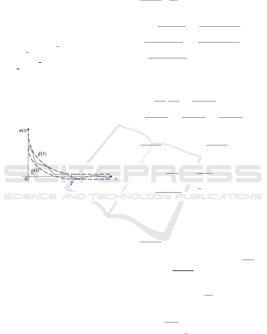
where

g(t)

and

(

)

are bounded functions with their

first time derivatives. These functions are chosen by

the designer based on the requirements of the system

operation.

For example (see Figure 1), one can guarantee

transients in a given tube whose boundaries

monotonically converge to the neighbourhood of zero

in a given time 𝑇. The description will be clearly

demonstrated in the appendix at the end of the paper.

Figure 1: An illustration of output error.

3 SOLUTION

Let us represent the operators in (1) as the following

sums:

(), ()() () ,

Rp Q QpR pQ

R =+ =+ΔΔ

(3)

where 𝑅



(𝑝) and 𝑄



(𝑝) are known differential

operators of orders m and n, respectively, and 𝑅



(𝜆)

and 𝑄



(𝜆) are Hurwitz operators, 𝛥𝑄

(

𝑝

)

and 𝛥𝑅

(

𝑝

)

are polynomials of orders not exceeding 𝑛−

1 and 𝑚 − 1, respectively.

For plant (1), we define a reference model of the

form

( ) () ( ) (),

mm mmr

Qpyt kRpgt=

(4)

Let the control law be

() ( ) (),ut T p t

(5)

where T(p) is chosen so that the transfer function





()()





()





has unit relative degree. Considering

(3), (5), let us rewrite (1) as

()() ()() ()

() ()

()() () ()()

()() ()() ()

() ()

() ()() () ()()

()()

(),

() ()

)

()

(

mmm

mm mm

kR p T p kR p T p R p

QpTp QpRpTp

kR p T p kR p T p Q p

tyt

QpRpTp QpRpTp

kR p T p

QpRpTp

∈

−+

(6)

where



(𝑡)

is the exponentially decaying function

due to nonzero initial conditions.

Substituting (5) into (6), we obtain

1()

() ()

() ()(

(

)

() 1 1

() () () .

()() ()() ()()

)

mm m

p aTp R pTp

yt f t t

RpTp RpTp R

υυ

∈



+−





−







(7)

Having isolated the integer part in the summand



(



)





(



)



(



)

𝑦

(

𝑡

)

=с



𝑦

(

𝑡

)





(



)





(



)



(



)

𝑦

(

𝑡

)

, we

transform (7) to the form of

()

() () ()

()

(

()

)()(),

()()

ttyt

pa Rp

yt f t t

yt с

υυ

∈



+−

−







−+







(8)

where 𝑐



is the integer part remaining when dividing

Δ𝑄

(

𝑝

)

to 𝑅



(

𝑝

)

𝑇

(

𝑝

)

,𝑐



are coefficients of the

polynomial 𝛥𝑄



(

𝑝

)

, 𝑐



are coefficients of the

polynomial 𝛥𝑅(𝑝) taken with opposite sign. 𝑓

(𝑡) =







(



)

()

𝑓(𝑡) is a new bounded disturbance due to

the boundedness of the original function 𝑓(𝑡) and

Hurwitz polynomial 𝑅



(

𝜆

)

𝑇

(

𝜆

)

. 𝜁



(

𝑡

)







(



)

𝑣(𝑡)

and 𝜁



(

𝑡

)







(



)



(



)

𝑦(𝑡) represent the filtered

signals at the output of the respective systems. When

dealing with the tracking problem, we additionally

consider the filter 𝜁



(

𝑡

)





(



)

𝑔



(

𝑡

)

Given (7), let us rewrite (8) as

01 02

() () ()

() () () .

ссytytt

tf tс t

υζ

ζ∈



=−−−





−++



(9)

Let us introduce the notations

Adaptive Output Control with a Guarantee of the Speciﬁed Control Quality

503

0010203

,,,

() () () (), (),,

() () (),

TTT

cccc

yt g tt

et yt y t

ζζω











=−

(10)

where 𝑐



is the vector of constant unknown

parameters, 𝜔(𝑡) is the regression vector.

Taking into account (9) and (10), let us write the

dynamics of the error 𝑒(𝑡) as follows

() () () () ())(.

et aet k f tcttt

υω ∈



=− + − +







(11)

According to (Annaswamy, 1998) and (Furtat,

2021) to solve the control problem with given

constraints, we introduce a replacement of the output

variable 𝑦 in the form of

() ()

() ( (),)

te gt

et t t

=Φ =

(12)

where 𝜀(𝑡) ∈ ℝ is a continuous-differentiable

function with respect to 𝑡,Φ(𝜀,𝑡) satisfies the

following conditions:

(a)

(

𝑡

)

<Φ𝜀

(

𝑡

)

(𝑡) for any 𝑡≥0 and

𝜀(𝑡) ∈ ℝ;

(b) there exists an inverse mapping 𝜀(𝑡) =



(𝑒,𝑡) for any 𝑒∈𝐸 and 𝑡≥0;

differentiable with respect to 𝜀 and 𝑡 and

(,)



≠0

for any 𝑒∈𝐸 and 𝑡≥0;

(d) the function

(,)



is bounded at 𝑡≥0 for any

𝜀

(

𝑡

)

∈ℝ. In that case

(,)







(



)

(



)



according to

(12).

Now let us determine the dynamics on the variable

𝜀 to investigate the stability of the closed-loop system.

For this purpose, we find the full time derivative of

(12) as

(,) (,)

() .

εε

∂Φ ∂Φ

∂∂



Since

(,)



≠0, taking into account (12), let us

rewrite the last equality as

(

(,)

()() ()

(,)

() () .

ae t t t

ευω

∈

−

∂Φ





=−+−





∂



∂Φ





++ −





∂





(13)

That is, by using the coordinate transformation

(13), the original problem with constraints is reduced

to a problem without constraints. Now it is necessary

to synthesise a control law 𝑢 that provides input-state

stability of the system (11).

Suppose that the derivatives of 𝑒(𝑡) are available

for measurement. Let us define an estimation of

axillary control signal 𝑣

(

𝑡

)

. Then consider the control

law in the form of

() ( ) ()

() () ()

()

1(,)

() ,

ut T p t

tttaet t

υω αε

∂Φ





=+−





∂







(14)

where 𝑐(𝑡) is bounded vector of adjustable

parameters, 𝑎>0.

Substituting (14) into (13), we obtain

()

(,)

() () () .()()

ttftcc t

εαεω∈

−

∂Φ







=−+ +







∂



−+



(15)

Let us formulate a theorem, the result of which

will be valid with the assumption that the derivatives

of 𝑦(𝑡) are measurable.

Theorem 1: Let the conditions (a)-(d) be satisfied,

Ф

(

,

)



for any 𝜀 and 𝑡, and 𝑠𝑢𝑝

Ф

(

,

)



<∞ and the

derivatives of 𝑒(𝑡) are measurable for the

transformation (12) and bounded. Then for any 𝛼 >

0,𝛽 > 0,𝛾 > 0, the control law (14) together with

the adaptation algorithm

(,)

() () () ()

ct t t с t

βεωγ

−

∂Φ



=− −



∂





(16)

guarantees that the output error signal 𝑒(𝑡) belongs to

the set (2).

Let us rewrite the control law (14) taking into

account that the derivatives of 𝑒(𝑡) are not

measurable:

ICINCO 2025 - 22nd International Conference on Informatics in Control, Automation and Robotics

504

() ( ) ()

()

() () ()

()

() ( )

1(,)

() .

, , ..., ,

ut T p t

tLt

tGtD t t

tttaet t

υξ

ξξ υυ

υω αε

μμ

−

=+ −

∂Φ



=+−



∂











=− − −













(17)

where the numbers 𝑑



,…,𝑑



are chosen so that the

matrix 𝐺=𝐺



−𝐷𝐿 is Hurwitz, 𝐷



𝑑



,…,𝑑



,𝜇 > 0 is a sufficiently small number.

Let us introduce vectors

𝜃



(𝑡)=𝑣(𝑡),...,𝑣

()

(𝑡) and 𝜂

(

𝑡

)

=𝛤



𝜉

(

𝑡

)

−

𝜃

(

𝑡

)

, 𝛤 = 𝑑𝑖𝑎𝑔



𝜇



,...,𝜇,1



Finding the derivative of 𝜂

(

𝑡

)

, we obtain

()

(), (

)()(() () ().)tGtb Lttttt

ηη μηυ

υυυ

−

Δ=−==−



(18)

Let us rewrite the equation with respect to the output

𝛥𝜐(𝑡):

(), ()

() () ().ttG Lttb t

ηη υ

υμη

−

Δ==−





(19)

Here

(1)

() () , 2,..., 1,

( ) ( ), [1 / ,0,...,0]

()/

tt i

ηη μ γ

ηη

−

=− = −



Then, based on the control law (17), we reduce the

error equation (16) to the form

() () () ()

())() (.

et aе tk t t

ft t

kL t

∈η

−



=− + −





++ +





(20)

Theorem 2: Let the conditions (a)-(d) be satisfied

for the transformation (17),



(

,

)



>0 for any 𝜀 and

𝑡, and 𝑠𝑢𝑝

Ф

(

,

)



<∞ and the derivatives of 𝑒(𝑡)

are not measurable. Then there exists such 𝜇<𝜇



that for any 𝛼>0,𝛽>0,𝛾>0, the control law (17)

together with the adaptation algorithm (16)

guarantees that the output error signal e(𝑡) belongs to

set (2).

4 EXAMPLES

Consider the plant (1) with Q(p) and R(p) given in the

form of

() ( ) ()

1 и 3,Qp p Rp=− =

The disturbance is represented as 𝑓(𝑡) = 7+

5𝑠𝑖𝑛(3𝑡)+4𝑐𝑜𝑠(2𝑡)+𝑑(𝑡), where 𝑑

(

𝑡

)

𝑠𝑎𝑡𝑑



(

𝑡

)

, 𝑠𝑎𝑡



⋅



is the saturation function, 𝑑



(𝑡) is

white noise modelled in Matlab Simulink using the

‘Band-Limited White Noise’ block with a noise

power of 1 and a sampling period of 0.2. The

disturbance is passed through a first order aperiodic

filter for smoothing. The graph of the disturbance is

shown in Figure 2a.

The reference model is given in the form

(), () 5cos(1.7 3)sin(0.5).

(1)

()

rrm

tgt t t

yt =

We choose 𝑇

(

𝑝

)

=𝑝+1. Hence the number 𝑎 in

(17) is 1, and the filters 𝜁(𝑡) take the form:

() , () .

ζζ

One filter is eliminated since

deg 𝑅



(𝑝) = 0.

The regression vector is then equal to

,,() () () (), () ,

ttttygt

ζζω









Let's form the control action (17) as

() () ()

()

() ( )

0.01

1(,)

() ,

tt tt

tttaet t

ξξ ξυ

υω αε

=− −

∂Φ





=+−





∂







In (2) we define

𝑔̄(𝑡) = 5𝑒

.

+0.3, 𝑔

(𝑡) =

0.2𝑒

.

−0.3. In the control law we set 𝑎=1,𝛼=

and 𝑘=1. In the adaptation algorithm (16), we

choose

𝛽=10 and 𝛾=10. The initial conditions

𝑦

(

)

=𝑦



(

)

. We take all other initial

conditions in the closed-loop system as zero.

Figure 2 shows the graphs:

disturbances (a), control

signal (b), output signal (c), control error

𝑒(𝑡)

transient with limiting functions (d).

Adaptive Output Control with a Guarantee of the Speciﬁed Control Quality

505

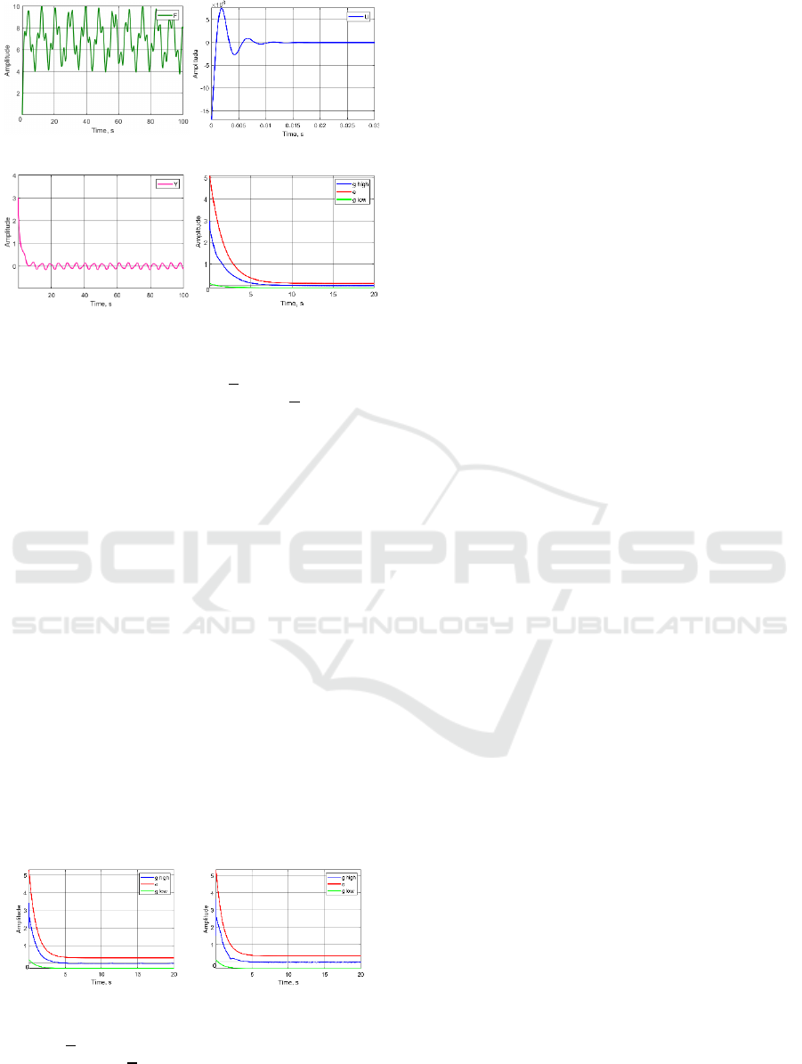
a) b)

)

Figure 2: Plant 1 - a) graph of disturbances; b) graph of

control signal; c) graph of output signal; d) graph of output

signal error with limiting functions

𝑔

(

𝑡

)

and 𝑔

(

𝑡

)

, defining

the quality of transient.

The advantage of the proposed algorithm, in

contrast to (Chopra, 2008), (Campion, 1989),

(Gerasimov, 2015) and other classical algorithms is

obvious: the transients are always contained in the

tube (2), the boundaries of which can define the

quality of the transients. Thus, the obtained processes

almost exponentially decay to the limit set (-0.1; 0.1)

in time 1.5 s., while the algorithms mentioned above

are not controllable in terms of transient process and

transient process time, as well as it is impossible to

determine a priori the quality of the output variable in

steady state.

As an example, consider the plant (1) with other

parameters:

() ()

4 +2 1 and 2,

+6 8 6 and 1.5 0.5.

Qp p p p Rp

Qp p p p Rp p

=− − =

=−+ =+

The error of the systems are shown in Figure 3 (a)

and (b) respectively.

)

Figure 3: Graphs of the output signal error with limiting

functions

𝑔

(

𝑡

)

and 𝑔

(

𝑡

)

: a) plant 2; b) plant 3.

5 CONCLUSIONS

In this paper, the methods of classical adaptive

control (Fradkov, 1999) and the method of nonlinear

control (Annaswamy, 2021) are applied, which

allowed us to create a new method of adaptive control

that guarantees a given quality of transient throughout

the whole process. At first, the new method is used to

transform the problem with constraints to a problem

without constraints. Then the classical method of

adaptive control is applied.

The simulation results confirmed the theoretical

conclusions and showed that in classical adaptive

control schemes at different parameters of the plant,

significantly different uncontrolled transient are

observed, while in the new control scheme at the

same parameters, the almost given quality of

transients is guaranteed.

ACKNOWLEDGEMENTS

The research was carried out with support of the grant

of the Russian Science Foundation № 25-19-20075,

https://rscf.ru/project/25-19-20075/ in IPME RAS.

REFERENCES

Annaswamy, A. M., Fradkov. A.L, (2021). A Historical

Perspective of Adaptive Control and Learning.

Annual

Reviews in Control, 52

, 18–41.

Arslan, G., Basar, T. (2001). Disturbance attenuating

controller design for strict-feedback systems with

structurally unknown dynamics.

Automatica, 37(8),

1175–1188.

Brusin, V.A. (1994) On a class of singularly disturbed

adaptive systems.

Avtomat. i Telemekh., 1995, no. 4,

119–129; Autom. Remote Control,

56:4 (1995), 552–

559.

Campion, G., Bastin, G. (1989). Analysis of an adaptive

controller for manipulators: Robustness versus

flexibility.

Systems & Control Letters, 12(3), 251–258.

Chopra, N., Spong, M. W. (2008). Output synchronisation

of nonlinear systems with relative degree one. In

Recent

advances in learning and control

(Vol. 371, pp. 51–64).

Springer. https://doi.org/10.1007/978-1-84800-155-8_4

Farza, M., M'saad, M., Maatoug, T., & Kamoun, M. (2009).

Adaptive observers for nonlinearly parameterised class

of nonlinear systems.

Automatica, 45(10), 2292–2299.

Fradkov, A. L., Miroshnik, I. V., & Nikiforov, V. O. (1999).

Nonlinear and adaptive control of complex systems.

Nauka.

Furtat, I. B. (2013). Robust synchronisation of the structural

uncertainty nonlinear network with delays and

disturbances.

IFAC Proceedings Volumes, 46(11), 227–

ICINCO 2025 - 22nd International Conference on Informatics in Control, Automation and Robotics

506

232. https://doi.org/10.3182/20130703-3-FR-4038.000

Furtat I., Gushchin P. (2021) Nonlinear feedback control

providing plant output in given set.

International

Journal of Control

. https://doi.org/10.1080/002071

79.2020.18613

Furtat, I., Gushchin, P., Nguen B. (2024) Nonlinear control

providing the plant inputs and outputs in given sets.

European Journal of Control 76(9)

10.1016/j.ejcon.2023.100944

Gerasimov, D. N., Lyzlova, M. V., & Nikiforov, V. O.

(2015). Simple adaptive control of linear systems with

arbitrary relative degree.

2015 IEEE Conference on

Control Applications (CCA)

, 1668–1673.

https://doi.org/10.1109/CCA.2015.7320849

Gnucci, M., & Marino, R. (2021). Adaptive tracking control

for underactuated mechanical systems with relative

degree two.

Automatica, 129, 109633.

https://doi.org/10.1016/j.automatica.2021.109633

Ioannou, P. A., Sun, J. (2012).

Robust adaptive control.

Courier Corporation.

Khalil, H. K. (2002).

Nonlinear systems (3rd ed.). Prentice

Hall.

Narendra, K. S., Annaswamy, A. M. (2012).

Stable

adaptive systems

. Courier Corporation.

Tsykunov, A. M. (2015). Robust control of a plant with

distributed delay.

Control Sciences, 76, 721–731.

APPENDIX

Proof of Theorem 1. Let us define a Lyapunov

function of the form

()()

()

((),)

()

ccc

∈

−

∞

=+ − −+



∂Φ



∂





(A1)

where

𝐻 > 0. Let us find the full time derivative of

(A1) using expressions (13) and (15). As a result, we

obtain

()

(,)

() () ()

(,)

().

Vtkftkt

kcccH t

εαε ∈

γε

∈

βε

−

∂Φ





=++−





∂



∂Φ



−−−



∂



−





(A2)

Let us use the following estimates from above and the

relation:

() ()()

() () 0,5 () () ,

0.5 .

TTT

tft t f t

tt t

cc c

сссccc cc

εεν

ε∈ ε ν∈



≤+







≤+









−= − −+−





(A3)

Given (A3), let us evaluate (A2) in the form

{}

()()

(,) 1

() 0,5 () sup

0,5 ( ) ( ) ( )

Vtktf

kttHt

k сс сс сс сс

αε ε ν

εν

εν∈ ∈

γγ

ββ

−

∂Φ 

  

≤−+ ++

  



∂

  







++−−











−−−++





It follows from the previous equation that if the

conditions are fulfilled

{}

()

Ф,

0,5 sup 0,5 sup

0,5

kf kHс c

ν∈ν

βε



∂

+−+



∂





−





the derivative of the Lyapunov function will be

negative. Thus, it is clear from the equation that there

always exist α and H that ensure this condition. It

follows from condition (b) that the transformation

(15) guarantees the fulfilment of condition (2). As a

result, function

𝑉 is bounded and therefore C is

bounded. Theorem 1 is proved.

Proof of Theorem 2. Let us rewrite equations (19),

(20) in the form:

() () () ()

(),

() (),

()

)

() ()

(

((

)

)),

с ket aе tLt

ktftt

ct t t

с t

μη

μη η

ω∈

βεωγ

−



=− + + +



∂Φ



=− −



∂



=−









(A4)

where

𝜇



=𝜇



=𝜇. Let us use the lemma (Brusin,

1994).

Lemma (Brusin, 1994). If a system is described by

equation

𝑥 =𝑓

(

𝑥,𝜇



,𝜇



)

,𝑥∈𝑅,

where 𝑓

(

𝑥,𝜇



,𝜇



)

is a continuous function that is Lipschitz on

𝑥, and at

𝜇



=0 has a bounded closed dissipativity area 𝛺





𝑥

𝐹

(

𝑥

)

<𝐶



where 𝐹

(

𝑥

)

is a positively defined,

continuous piecewise smooth function, then there

exists such

𝜇



>0 that at 𝜇



<𝜇



the original

system has the same dissipativity area

𝛺



if for some

Adaptive Output Control with a Guarantee of the Speciﬁed Control Quality

507

numbers 𝐶



and 𝜇̅



with 𝜇



=0 the following

condition is fulfilled

()

sup ( , ,0) ,

μμ

≤



∂



≤−



∂



(A5)

when 𝐹

(

𝑥

)

=𝐶.

Let us take the Lyapunov function



η



(

)



η

(

)





>0 is determined from the

solution of the equation



G+G





=−Q



, where





>0, then considering (A.4) we obtain 𝑉





−







η



(

)





(

)

with μ



=0. It means that at 𝜇



we obtain the original equations (11), (16) to which

we add the independent equation

𝜇



𝜂̅



(

𝑡

)

=𝐺𝜂̅

(

𝑡

)

with asymptotically stable variable

𝜂̅

(

𝑡

)

. Hence, for

the initial system we have a dissipativity region

𝛺

with an attraction region

𝛺



Let us take the Lyapunov function as a function

𝐹(𝑥)

() () () () ()

() () () (),

Fhet ctct tH t

tH t tH t

υυ

ζζ

ζζηη

=+ + +

(A6)

where ℎ



>0, 𝐻



,𝐻



,𝐻



are positively defined

symmetric matrices.

Let us set the number C such that the surface

𝐹

(

𝑥

)

=𝐶, where 𝑥



(

𝑡

)

=𝑐,𝜂̅



,𝜁





,𝜁





 is boundedly

closed, is in the area

𝛺 on the variables 𝑥

(

𝑡

)

, and

since the set

𝛺



lies in the open area 𝑉

(

𝑥

)

<𝐶 and

the system is dissipative, the variables

𝑥

(

𝑡

)

will tend

to attraction area

𝛺



, and hence there exists a number

𝐶



for which (A5) is satisfied. The rate of

convergence of the variables

𝜂̅

(

𝑡

)

to zero will depend

on the choice of

𝜇



. Therefore, according to the

lemma (Brusin, 1994), there exists

𝜇



>0 such that

𝜇<𝜇



the dissipativity area of the system (17),

(19), (20) remains the area

𝛺. Theorem 2 is proved.

ICINCO 2025 - 22nd International Conference on Informatics in Control, Automation and Robotics

508