
Comparison of the Hubble Tension Measurement from Two
Approaches: Distance Ladder and CMB
Shuowen Qian
King’s School Canterbury, Canterbury, U.K.
Keywords: Hubble Constant, Hubble Parameter, Hubble Tension, Distance Ladder, CMB.
Abstract: The Hubble Tension arose when two distinct values of the Hubble constant were calculated, which implied
either experimental flaw, or a fundamental misunderstanding of the universe. This study provides an overview
of the mathematical meaning of the Hubble constant using Hubble’s Law, as well as the Hubble parameter by
interpreting the terms in the Friedmann Equation. The distance ladder method will also be elaborated; by
explaining the basic mechanism of the method, which is observing the absolute magnitude of the Cepheid
variable stars, calibrating them with the Type la Supernovae, eventually establishing a correlation where
distance increases linearly with velocity, in which the Hubble constant is the constant of proportionality. The
CMB method will be explained particularly with the underlying features of CMB that enable this method: the
BAO and the sound horizon, which is integrated into the method of inputting observed values from the angular
power spectrum into the ΛCDM to generate Hubble constant. Comparisons, limitations, of the two methods
will be addressed, such as the interference to observation by the metallicity of Cepheids dense star-forming
regions, the reliance on Cepheids of the Type la Supernovae in the distance ladder method. The sensitive
dependence on the ΛCDM model; as well as the potential incompleteness of the model for the CMB method.
A further discussion of the scientific meaning of Hubble tension will also be provided.
1 INTRODUCTION
The understanding of the Universe has been greatly
expedited during the 20th century. Einstein’s creation
of General Relativity, followed by his own solutions
to the Einstein Field under the assumptions of a
spatially homogeneous and isotropic universe by
introducing the cosmological constant Λ. Einstein’s
solution models the Universe as perfectly static; that
is neither expanding nor contracting, where Λ
counteracts the attraction of gravity.
In 1922 Friedmann proposed a new set of solution
to Einstein’s Field, one that does not rely on the static
nature of the Universe, that the Universe is either
expanding or contracting, despite the mathematical
solution did not receive any observational proof until
1929. In 1929 Hubble measured the distance of the
Milky Way to nearby galaxies using Cepheid
Variables, as well as the redshift of light emitted from
those galaxies and discovered that the expansion
velocity of the galaxies is linearly proportional to the
distance, expressed as:
(1)
where
is the Hubble Constant (Hubble 1929)
Hubble’s discovery reveals that the further a galaxy
is, the faster it is receding away from the observer,
which means the universe is expanding, as well as the
space between neighbouring galaxies. As if all
galaxies are mapped on to specific points on a fabric
of elastic rubber, as the rubber stretches, the relative
distance between two points also increases.
Hubble’s discovery lies in the heart of modern
cosmology, as it sheds light onto the rudimentary
configurations of the Universe, such as age, the past,
present and future of the universe. Though the two
most popular methods in calculating
– via cosmic
distance ladder and cosmic background radiation -
show discrepancies in their values, know as the
Hubble Tension.
More precise measurement of the Hubble constant
in recent years show discrepancies between two
fundamentally different methods – the distance ladder
and CMB. The major difference between the two
methodologies is that the CMB method does not
measure the Hubble constant directly, instead a value
for Hubble constant is inferred from the ΛCDM
simulation from modelling the Universe during the
Epoch of Recombination(Yadav 2023). On the other
240
Qian, S.
Comparison of the Hubble Tension Measurement from Two Approaches: Distance Ladder and CMB.
DOI: 10.5220/0013822800004708
Paper published under CC license (CC BY-NC-ND 4.0)
In Proceedings of the 2nd International Conference on Innovations in Applied Mathematics, Physics, and Astronomy (IAMPA 2025), pages 240-245
ISBN: 978-989-758-774-0
Proceedings Copyright © 2025 by SCITEPRESS – Science and Technology Publications, Lda.

hand, the distance ladder offers direct mathematical
measurement and computation from the preset-day
universe.
The SH0ES collaboration, via the distance ladder
method, measures the luminosity of the standard
candles (Cepheids and 1a Supernovae) through which
the Hubble constant can be calculated through
measuring distance and redshift. SH0ES incorporates
their research with data from Gaia and Hubble Space
Telescope, sets the value of the Hubble constant as
(Riess 2022).
On the other hand, the Planck satellite utilises the
CMB method which focuses on measuring the
temperature fluctuations thus calculating the Hubble
constant by extrapolating distance from the measured
angular size of the sound horizon. These fluctuations
are then plotted on an angular power spectrum which
is modelled in the ΛCDM simulation, through which
the Hubble constant is inferred. The value of the
Hubble constant is found to be
(Planck 2018).
The initiative of this paper is to deliver a generic
overview of the Hubble tension, starting from the
foundations of the Hubble constant as the theoretical
implication in determining the configurations of the
Universe. Analysis of the experimental approaches of
measuring the Hubble constant that give rise to the
Hubble tension; particularly from the cosmic distance
ladder and CMB methods, by accessing data from
pre-existing academic establishments and publicly
accessible data such as the Planck satellite. The
following parts will be comprised as follows. An
explanation to the principles of the Hubble constant
and Hubble parameter. A description of the distance
ladder method, how Hubble constant is measured
using distance ladder, as well as the relevant data
analysis such as the Period-Luminosity relation.
Subsequently, a description of the CMB method, and
relevant approaches in measuring Hubble’s constant,
and the dependence of the ΛCDM. Afterwards, a
comparison of the two values, a discussion of other
methods, as well as prospects that would possibly
explain the existence Hubble tension, or possible
resolution.
2 PRINCIPLES OF THE HUBBLE
LAW
The Hubble constant describes the current rate at
which the universe is expanding. It displays a linear
relationship between the recessional velocity of the
galaxy and the distance from the observer. The
recessional velocity unit of the Hubble constant –
km/s/Mpc indicates that the recessional velocity of
the galaxies increases by a value of
for every
megaparsec of separation.
This increase in velocity does not imply the
galaxies are ‘moving through’ space, but the
stretching of the space itself, where galaxies
consequently separate out from one another. Taking
the analogy of the balloon, the galaxies, as dots on the
balloon as it is to space; as the balloon expands, the
dots move apart from each other, this is analogous to
the separation of the galaxies from one another.
Therefore, the cosmological redshift is strictly due to
the geometric phenomenon of the space expanding,
distinctively dissimilar to the Doppler effect in
Kinematics (Peacock 1999).
From the equation above, given the Hubble
constant at the present time, the age of the universe
can be approximated as
≈
(2)
where the age of the universe is approximately 13.8
billion years, this equation is a mere estimation, and
further detail will be provided in Part 2. The Hubble
constant marks the crucial relationship in converting
observed cosmological redshift into physical
distances. It is also instrumental in producing large-
scale maps of the universe, as well as marking the
boundary conditions for computational simulations,
such as the ΛCDM (Riess 2022).
The Hubble parameter
defines the
expansion rate of the universe as a function of time.
It is given by the ratio of the time derivative of the
scale factor
. Here,
describes the size of the
universe at a given time, where the scale of the
universe at any time is a ratio to the present time
. Therefore, at
is the future and
the past. The derivative of
Indicates
the instantaneous change of the size of the universe
with respect to time. Thus,
can also be defined as:
(3)
Following from Part 1, a more refined, accurate
computation of the age of the universe, as the Hubble
constant does not represent the uniform rate of
expansion across the entire time duration, the more
accurate age of the universe will be the integral of the
Hubble parameter for all values of . The Hubble
parameter is determined by the energy distributions in
space, expressed as the Friedmann Equation
(Friedmann 1922):
(4)
where the Hubble parameter is dependent upon the
energy density at any given time
expands to
give:
Comparison of the Hubble Tension Measurement from Two Approaches: Distance Ladder and CMB
241
(5)
In which the radiation and matter density at a given t
is inversely proportional to their density at
,
therefore the overall energy density decreases as
, increases when
relative to the
current age of the universe, where as the dark matter
density remains constant over time, this is also why
the present universe is a dark matter-dominated
universe (Weinberg 1972). The relative energy
densities of radiation and density are “mass-constant”,
therefore the total quantity of radiation and matter
remain constant, whereas dark energy is “density-
constant”, therefore the total dark energy existing
increases as the universe expands.
The second term
describes the spatial
curvature of the universe, where k takes values of
either -1, 0, +1, reflecting the universe being open,
flat, or closed, though the numerical value assigned to
this mathematical term decreases asymptotically to 0
as
increases. The last term describes the
dark energy content in the universe, acting as though
a repulsive force through space. Due to the shifting of
significance and numerical scale of each energy
density at different epochs of the universe, which
implies that the change in the Hubble parameter was
not uniform. Therefore, integration is used for a more
accurate age of the Universe.
3 MEASURING H
0
VIA
DISTANCE LADDER
The distance ladder method is a direct way of
determining the Hubble constant. The process
involves calibrating stepwise using a series of
increasingly distant astronomical objects, where each
step of the ladder provides the foundation for the next.
The two most relevant standard candles for this
method are the cepheid Variable stars, and the Type
la Supernovae. These stellar objects are crucial to the
“Supernovae and
for the Equation of State” –
SH0ES’ collaboration work to refine their value for
the Hubble constant.
Cepheid variable stars are radially pulsating stars
characterised by a periodic variation in their
luminosity, as a result of their contracting and
expanding outer layer due to the inward gravitation
force. The correlation between the periodicity and
luminosity is given by the Period-Luminosity relation
discovered by Henriette Leavitt. This relation allowed
a direct way of determining luminosity, solely with
accurately measuring the duration of the varying-
luminosity period.
The proportionally between period and luminosity
was first discovered by Leavitt via observations of
Cepheid variables in the Small Magellanic Cloud.
The relation was later calibrated using Cepheid
variables within the Milky Way, whose distances
were measured in the parallax method, thus
establishing the scale between period and absolute
magnitude and anchoring the luminosity scale as
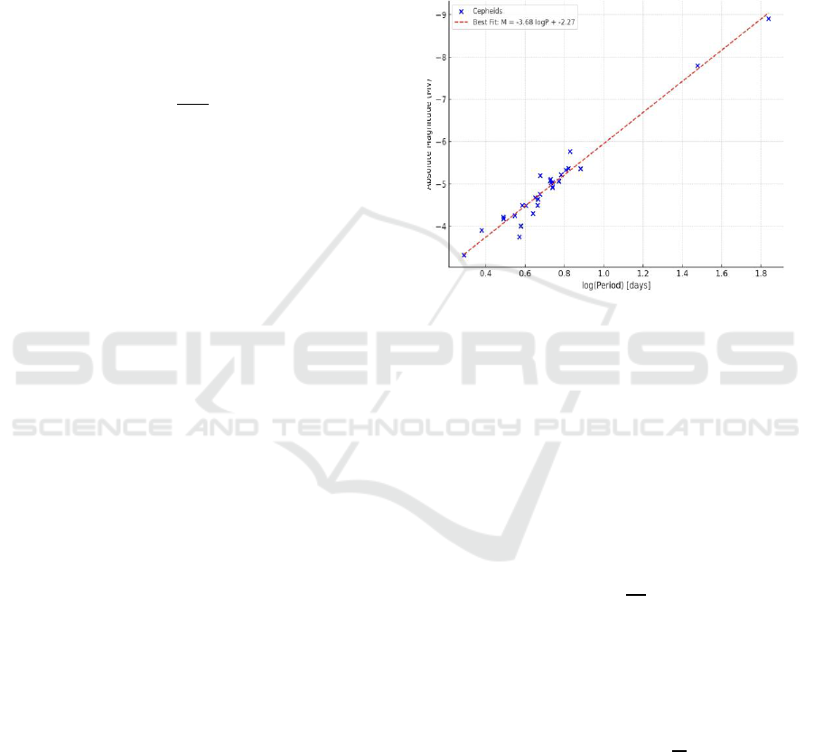
shown in Figure 1.
Figure 1: The linear relationship between periodicity
and absolute magnitude is displayed by the linearity of the
plotted line, which aligns with Leavitt’s discovery (Storm
J. 2011).
The proportionality is given by:
(6)
where is the absolute magnitude, the period in
days, the change in brightness with respect to
period, and the absolute magnitude when the period
is 1 day. The Gaia Space Observatory measured
parallax for nearby Cepheids with a precision of
below 1 milli-arcsecond (Gaia Collaboration 2021).
More massive and luminous Cepheids have lower
gravity,
(7)
This is because the increase in radius outweighs the
increase in mass, yielding a lower gravitational field
strength, this consequently increases the period of the
expansion and contraction process, thus the period
pulsation. By observing the absolute magnitude with
the observed magnitude, the distance is given by:
(8)
where is the apparent magnitude and the
absolute magnitude, where g is in parsecs. The
Cepheids are observed using the Hubble Space
Telescope, then calculating the red shift the
recessional velocity of the Cepheid can be found
using , thereby constructing a graph of
IAMPA 2025 - The International Conference on Innovations in Applied Mathematics, Physics, and Astronomy
242
velocity against measured distance, the gradient is
given to be the Hubble constant.
Despite the method via Cepheid variables being
straightforward, it is not without its flaws and
limitations. Cepheids variable stars are located in
dusty star-forming regions where extinction (the
reduction in intensity and scattering of light) occurs
frequently in the visible light spectrum. Therefore, the
F160W band is frequently used nowadays as the
subject of the detection, as the infrared radiation
emitted from F160W is hardly obscured by the
surrounding stars (Riess 2021).
Another limitation of the Cepheid variable stars
is their metallicity. Elements heavier than Hydrogen
and Helium will absorb radiation emitted by the
Cepheids, which changes the frequency of the light
received on Earth, this consequently leads to
miscalculations regarding the size of the Cepheid,
thus the distance, and the Hubble constant. This
becomes problematic when two Cepheids that have
the same period, mass, would lead to discrepancy and
inaccuracy over the calculated Hubble constant value,
therefore the inaccuracies must be mitigated using
spectroscopic analysis (Riess, 2021; Yuan & Riess,
2023]
Type la Supernovae becomes useful when
observing distant galaxies, where the distance is so
great that barely any radiation can be detected by the
Cepheid Variables. Type la supernovae are the
thermonuclear explosions of carbon-oxygen white
dwarfs in binary systems. Which occurs when a
carbon-white dwarf accretes mass from a companion
star mass, where nuclear fusion occurs for carbon and
oxygen, overcoming the outward electron degeneracy
pressure, which leads to an explosion. The explosion
produces a light curve with uniform luminosity and
shape, which is used to standardise the luminosity of
the Type la supernovae (Riess 2022).
Type la Supernovae are not intrinsically standard
candles, as their absolute magnitude cannot be
previously known, therefore the external calibration
of the luminosity of the la supernovae relies on
Cepheid variables acting as anchors. The calibrated
luminosity is inferred from a similar equation
(9)
On this basis, a similar graph of recessional velocity
vs. distance can be plotted, provided that the redshift
is negligible, in which the gradient is inferred as the
Hubble constant.
The most recent determination of the Hubble
constant via the distance ladder method is from Riess
et al. 2021, by observing over 1000 Cepheids and 42
Type la Supernovae across different host galaxies
(Riess 2021), which found the value to be
(10)
In 2022, the SH0ES collaboration reduced the
percentage uncertainty below 2% by using more
advanced calibration and a larger dataset
demonstrated the consistency of the Hubble constant
by measuring using different anchoring galaxies such
as NGC 4258, LMC and the Milky Way, the resultant
value for the Hubble constant remained consistently
above 72km/s/Mpc. (Riess, 2021; Yuan & Riess,
2023)
4 COMPUTING H
0
VIA CMB AND
ΛCDM
The CMB method measures the anisotropies in the
temperature map imprinted at the Epoch of
Recombination (380000 years). Anisotropies are
variations of temperature in regions of the CMB map,
as red displays higher temperature regions and blue
cold. The anisotropies reflect on the distribution of
different energy densities across different regions in
the primordial universe, as the result of the variations
in intensity of Baryon-Acoustic Oscillations
(oscillations of photon-baryon plasma), which are
imprinted on the angular power spectrum, which is
analysed within the ΛCDM model, computing
(Planck 2018). The Angular power spectrum
describes the temperature anisotropies specifically
from the Epoch of Recombination-when the photons
in the CMB had just become free from scattering with
electrons-using spherical harmonics. Spherical
harmonics break down temperature variations
observable in the CMB, correlating the temperature
variations to specific angular scales. Multipole
moment corresponds to angular scale, where a small
multipole moment means larger angular scale. The
peaks in the angular power spectrum indicate Baryon
Acoustic Oscillation.
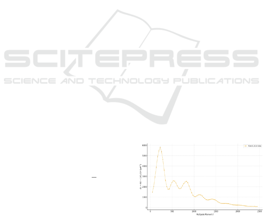
Figure 2: This is a graph displays the relation between
angular power spectrum with a range of multipole moments
(Planck 2018).
Comparison of the Hubble Tension Measurement from Two Approaches: Distance Ladder and CMB
243

As shown in Figure 2, the peak at
indicates
the most prominent first harmonic acoustic oscillation
in the photon-baryon plasma during the Epoch of
Recombination, signifying the largest complete
compression mode of the sound wave generated by
the oscillation. The oscillations lead to rarefaction
and compression in regions of the CMB as sound
waves. The sound waves then stop propagating at the
Epoch of Recombination, in which the freed photons
from the photon-baryon plasmas carry information of
these BAO, which then the photons are detected by
microwave telescopes (Planck, 2018 & Hu, 2022),
that indicate the temperature fluctuations of the CMB
around the Epoch of Recombination.
The sound horizon is the distance the sound waves
from BAO could travel before the Recombination,
where angular scale θ is the ratio between the sound
horizon and the angular diameter distance, which
measures the distance to the point where the photons
became free. The angular power spectrum and
multipole moments infer the angular size of the sound
horizon determine the angular size of the sound
horizon. Where the angular size of the sound horizon
is dependent on the expansion rate of the universe,
therefore dependent on the Hubble constant. A higher
expansion rate leads to smaller angular size, as
distance is further, and vice versa.
With the calculated angular size from the
observed CMB, the values are inserted into the
ΛCMB model, which computes a theoretical value of
the Hubble constant, by correlating angular size with
the rate of expansion (Planck 2018).
The development of the CMB method is reflected
by the three generations of satellites. The cosmic
background explorer COBE, 1989-1993 initially
detected the anisotropies of the CMB temperature,
and that the radiation spectrum of the CMB at 2.725K
adheres closely to the black body curve, which
implied that the early universe was uniform and in
thermal equilibrium, where matter and radiations
existed in a very hot and dense condition, the
uniformity implied the cooling and expansion of tue
universe over time, which aligns with the observed
evidence (Smoot 1992). The Wilkinson Microwave
Anisotropy Probe 2001-2010 improved the angular
resolution from 7 degrees to 0.2 degrees, yielding a
refined value of the Hubble constant
(11)
(Bennet 2013). The Planck mission 2009-2013
provided further observations of temperature
anisotropies to 2500 multipole moment, operating
closely with the ΛCDM, Planck mission yielded a
value of Hubble constant as
(12)
(Planck 2018).
The major limitation of the CMB method is that it
is heavily dependent on the accuracy of ΛCDM
model, the given parameters of dark energy, dark
matter, and baryonic matter within the model are
assumed to be accurate, which means any known, or
unknown deviations within this model, will compute
a different value for the Hubble constant (Di
Valentino 2021).
5 COMPARISON AND
PROSPECTS
The two methods both provide a logical, precise path
towards the derivation of the Hubble constant, though
they do not converge on an unequivocal result, but
differ by a difference of 5σ. The two methods
fundamentally disparage in a multitude of ways,
where the distance ladder observes the modern
universe, and the CMB method studies the early
universe at the Epoch of Recombination. The distance
ladder method being empirical and observation-based,
whereas the CMB method relies on a model. The two
methods could be subjected to inaccuracies in their
measurements, such as the metallicity of the Cepheid
variables which would obscure the measurements, or
the disproportionality of dark energy, dark and
baryonic mater within the configurations the ΛCDM
model. Another possible explanation might be the
lack of understanding of the ‘invisible’; perhaps dark
energy is not an invariable, but one that changes
according to the scale of the Universe, which might
yield a completely different and independent value of
.
Another independent method of calculating the
Hubble constant is by establishing a direct
relationship between the temperature of the CMB
with the Hubble constant, a mathematical model,
which is subjected to much less inaccuracy in
comparison with the distance ladder and CMB
method, relying only on the observed value for the
temperature of the CMB (Tatum 2024):
(13)
The Hubble constant calculated to be
which is very similar to the value computed by the
Planck mission. The Hubble tension not only displays
a fundamental difference in value via the two most
popular methods, but also a reflection of the unknown
of the universe. In the future more accurate values of
the Hubble constant will be calculated, with finer
IAMPA 2025 - The International Conference on Innovations in Applied Mathematics, Physics, and Astronomy
244

understanding of the universe, and more advanced
methods, though it is most crucial, to lay the
foundation for those methods by developing a finer
understanding of the ingredients of the Universe.
6 CONCLUSION
To conclude, this study serves as an overview of the
two observational methods of the Hubble constant –
distance ladder and CMB, and how they
fundamentally disagree with each other which results
in the Hubble Tension. This paper also delves into the
mathematical meaning of the Hubble constant and
Hubble parameter, as well as their significance in
relation to the age, expansion rate and the dynamics
of the universe, as though a blueprint on which all the
known and unknown knowledge of the universe is
imprinted. The empirical, observational fashion of the
distance ladder method, first by establishing a
correlation between period and absolute magnitude of
Cepheids and Type la Supernovae via parallax and
calibration, to find distance and calculate Hubble
constant, limited by the metallicity of Cepheids and
the dependent nature of the la supernovae. The
modelling method of the CMB via ΛCDM, by tracing
back to the very beginning of the universe, with data
of angular scale, size, multipole moment provided by
three generations of satellites, though considered
flawed due to the incompleteness of the ΛCDM
model. The Hubble constant is a reflection of the
rudimentary parameters that govern the universe. In
order to establish on a single unfalsifiable value of the
Hubble constant, the analysis of the configuration of
the universe is the most urgent task for modern
Astrophysics. Perhaps only by fully interpreting the
known knowledge and unchartered enigmas of the
Universe, will the infallible notion of the Hubble
constant be ultimately revealed.
REFERENCES
Bennett, C. L., Larson, D., Weiland, J., et al., 2013. Nine-
Year Wilkinson Microwave Anisotropy Probe (WMAP)
Observations: Final Maps and Results. The
Astrophysical Journal Supplement Series, 208(2), 20.
Di Valentino, E., Anchordoqui, L., Akarsu, Q., et al. 2021.
Cosmology intertwined II: The Hubble constant tension.
Astroparticle Physics, 131, 102605.
Friedmann, A. 1922. Über die Krümmung des Raumes.
Zeitschrift für Physik, 10(1), 377-386.
Gaia Collaboration, Brown, A. G. A., Vallenari, A., Prusti,
T., et al. 2021. Gaia Early Data Release 3: Parallax bias
versus magnitude, colour, and position. Astronomy &
Astrophysics, 649, A1
Hu, W., & Dodelson, S. 2002. Cosmic microwave
background anisotropies. Annual Review of
Astronomy and Astrophysics, 40, 171–216
Hubble, E., 1929. A relation between distance and radial
velocity among extra-galactic nebulae. Proceedings of
the National Academy of Sciences, 15(3), 168–173.
Peacock, J. A. 1999. Cosmological Physics. Cambridge
University Press.
Planck Collaboration. 2018. Planck 2018 results. VI.
Cosmological parameters. Astronomy & Astrophysics,
641, A6.
Planck Collaboration. 2020. Planck 2018 results. V. CMB
power spectra and likelihoods. Astronomy &
Astrophysics, 641, A5.
Riess, A. G., Yuan, W., Macri, L. M., et al., 2022. A
comprehensive measurement of the local value of the
Hubble constant with 1 km/s/Mpc uncertainty from the
Hubble Space Telescope and the SH0ES Team. The
Astrophysical Journal Letters, 934(1), L7.
Smoot, G. F., Bennet, C. L., Kogut, A., et al., 1992.
Structure in the COBE DMR first-year maps. The
Astrophysical Journal Letters, 396, L1–L5.
Storm, J., Gieren, W., Fouqué, P., et al. 2011. Calibrating
the Cepheid period–luminosity relation from the
infrared surface brightness technique. Astronomy &
Astrophysics, 534, A95.
Tatum, E. T., & Haug, E. G. 2024. Predicting High
Precision Hubble Constant Determinations Based on a
New Theoretical Relationship between CMB
Temperature and H0. Journal of Modern Physics,
15(11), 1708-1716.
Weinberg, S. 1972. Gravitation and Cosmology. Wiley.
Yadav, V. (2023). Measuring Hubble constant in an
anisotropic extension of ΛCDM model. Physics of the
Dark Universe, 42, 101365.
Yuan, W., Riess, A. G., Macri, L. M., et al. 2023.
Consistency of local H_0 measurements using
alternative calibrator galaxies. The Astrophysical
Journal, 946(1), 61.
Comparison of the Hubble Tension Measurement from Two Approaches: Distance Ladder and CMB
245
