Analysis and Prediction of TESLA Stock Based on the ARIMA Model

Jinghan Wang

School of Mathematical Sciences, Capital Normal University, Beijing, 100142, China

Keywords: Time Series Analysis, Stock Prediction, ARIMA Model, New Energy Vehicles.

Abstract: TESLA, as the leader in new energy vehicles, has set a record high in multiple transaction volumes and profits

in 2024. Accurate prediction of Tesla's stock prices is crucial for investors and market analysis. This article

will select TESLA's stock price in the past decade to conduct a series of time series analyses such as

stationarity test, difference, and residual test to build a suitable Autoregressive Integrated Moving Average

(ARIMA) model and use this to predict the stock price in the next five years, hoping to provide strong

decision-making support for the government, enterprises, and individuals to promote high-quality

development of the new energy vehicles industry. The final results show that the model has a relatively high

performance and shows an upward trend. Next, the possible reasons for this phenomenon were further

analyzed. However, because stock prices are affected by many factors, there may be large errors in making

predictions, and further, updating the model and in-depth research is needed.

1 INTRODUCTION

Tesla has occupied an important position in the

Electric Vehicle (EV) market, especially in key

markets such as the United States and China, and its

market shares and transaction volume have continued

to grow. According to Tesla's third-quarter financial

report in 2024, the Tesla Shanghai Energy Storage

Super Factory will be put into production in the first

quarter of 2025. The scale of energy storage is nearly

40 GWh, and its products are supplied to the global

market (Wu, 2024). However, as the traditional car

manufacturers enter the electric vehicle market, Tesla

faces increasingly fierce competition. To cope with

the pressure, Tesla has implemented a package of

promotional measures worldwide (Xi, 2024).

The high volatility and complexity of Tesla’s

stock make it a typical case of financial market

research. Mao (2020) used a time series-based

combinatorial model to predict CPI in Jiangxi

Province. The results show the prediction effect of

using a combined model is better than that of a single

model. Based on evaluating the model fitting effect,

Xiao (2024) predicted the per capita disposable

income of rural permanent residents in Jiangsu

Province. Jiang (2015) analyzed and predicted the

stock of Baogang, proving the effectiveness of the

https://orcid.org/0009-0000-1410-4589

experimental results. Zhang (2020) introduces the

development history and research of time series and

stock forecasts and explains the concepts and

common methods of time series.

Stock prices are typical time series data with

obvious periodic characteristics. At present, no

predictions have been given by the Autoregressive

Integrated Moving Average (ARIMA) model.

Previous researchers only have the general analyses

of its stock at key nodes, which are relatively shallow

and at a single level. So, this article will give forecast

data for nearly 5 years by ARIMA model, which can

be further used to explore the pricing mechanism and

market behavior of stocks of new technology

companies. The analysis and prediction of Tesla

shares in this article can help investors understand the

risks and income characteristics better, thereby

making wise investment decisions. Meanwhile,

Tesla's stock performance reflects the overall trend of

its industry, which can help deeply understand the

development dynamics of the EV industry, and

provide data support for policymakers.

Wang, J.

Analysis and Prediction of TESLA Stock Based on the ARIMA Model.

DOI: 10.5220/0013813600004708

Paper published under CC license (CC BY-NC-ND 4.0)

In Proceedings of the 2nd International Conference on Innovations in Applied Mathematics, Physics, and Astronomy (IAMPA 2025), pages 37-41

ISBN: 978-989-758-774-0

2 METHODOLOGY

2.1 Data Source

The data used is from the website Kaggle

(https://www.kaggle.com), which is a reliable data

science platform with data sets strictly screened and

preprocessed to ensure quality and availability. The

dataset includes the DATE: the date of stock data, the

HIGH: the highest price that Tesla stock reached on

that date, and the LOW: the lowest price that Tesla

stock has reached on that date from 2015 to 2024.

This article will use the average of the highest and

lowest selling prices to represent the price of the day.

Data from 2015-2024 can be used as training, and

then predict the next 5 years.

2.2 ARIMA Model Introduction

Stock prices are typical time series data with obvious

periodic characteristics. The ARIMA model is a

classic time series model suitable for stationary or

approximately stationary time series data, which can

capture these features and adapt to different time

series data characteristics by adjusting parameters.

This flexibility allows it to fit the stock price change

pattern better.

ARIMA model combines 3 parts: autoregression

(AR), differential (I, Integrated), and moving average

(MA). AR represents the linear relationship between

the current observation value and the past observation

value. An AR model contains one or more lag terms,

and their coefficients represent the effects of those

past values on the current value. I mean stabilizing the

data by differentiating the original time series because

the smooth time series are easier to model. The

difference order is used to indicate the times that

difference is required to stabilize the data. MA

represents the linear relationship between the current

observation value and the error of the past

observation value. An MA model contains one or

more lagged error terms, and their coefficients

represent the effect of past errors on the current

observation. It’s usually expressed as ARIMA (p, d,

q), where p is the autoregressive order (the number of

lag terms in AR), d is the difference order (the number

of times of difference), and q is the moving average

order (the number of lag terms in MA). The modeling

process of the ARIMA model includes selecting

proper p, d, and q values, fitting the model, and

analyzing the residual (Zhou, 2024).

3 RESULTS AND DISCUSSION

3.1 Stationarity Test

The ARIMA model requires that the time series be

stationary, so the first step is to conduct a stationary

test on the original data. If the stationary test cannot

be passed, it means that the data contains some time

or periodic trend. The most intuitive method is to

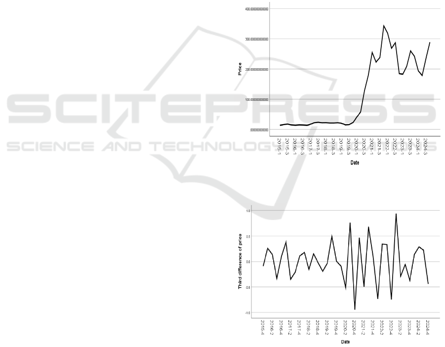
observe the line chart in Figure 1, and you can find

that the original sequence is unstable. Tesla's shares

Prices were relatively stable between 2015 and 2019

and rose sharply between 2020 and 2024. By

performing first-order and second-order differences

on the data, it was found that the data still did not pass

the stationarity test until the third difference. The

third difference result is shown in Figure 2.

Figure 1: Tesla’s stock price change line chart from 2015

to 2024 (Photo/Picture credit: Original).

Figure 2: The third-order difference of Tesla’s stock price

(Photo/Picture credit: Original).

To perform stationarity tests on a given data, we

can use the Unit Root Test, the most commonly used

is the ADF (Augmented Dickey-Fuller) test (Zuo,

IAMPA 2025 - The International Conference on Innovations in Applied Mathematics, Physics, and Astronomy

2019). The null hypothesis (H0) of the ADF test is

that the sequence has a unit root; that is, the sequence

is not stationary. The alternative hypothesis (H1) is

that the sequence has no unit root; that is, the

sequence is stationary. Since ADF statistic -3.214 is

less than the critical value of -2.92 at the 5% level,

and the p-value is 0.019 less than 0.05, it rejects the

null hypothesis. Therefore, the data after the third-

order difference is stationary. So it can pass the

stationary test.

3.2 Construction of the ARIMA Model

The formula of the ARIMA model is:

∆



𝑋



=𝛼



𝑋



+𝛼



𝑋



+...+𝛼



𝑋



𝜀



+𝛽



𝜀



+𝛽



𝜀



+...+𝛽



𝜀



, (1)

where ∆



represents a stationary sequence after d-

order differentiation of time series 𝑋



, 𝛼



, 𝛼



,..., 𝛼



is the coefficient of the autoregressive part. 𝛽



, 𝛽



,...,

𝛽



is the coefficient of the moving average part. 𝜀



a random error term. p and q are the orders of

coefficients in formula (1). And d is the order of the

difference.

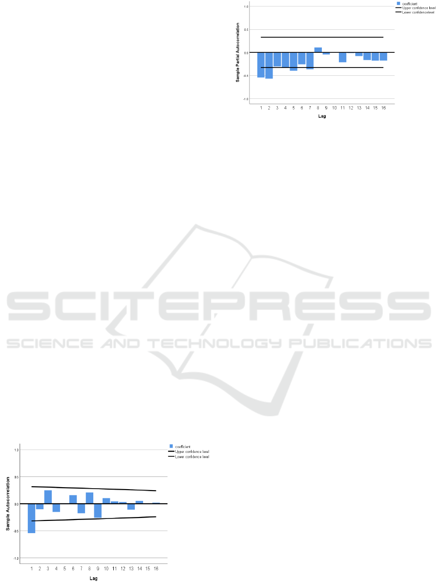
To determine this parameter, the common method

is the autocorrelation function (ACF) and partial

autocorrelation function (PACF). Figure 3 is the ACF

graph. The horizontal coordinate represents the lag

order, which is the time interval between the current

value and its lag value in the time series, while the

ordinate coordinate represents the autocorrelation

coefficient and is the intensity of the correlation

between the current value and the hysteresis value.

And Figure 4 is the PACF graph. The meaning of the

horizontal coordinate is the same as the ACF graph.

The vertical coordinate represents a PACF

coefficient, which is the pure correlation between the

current value and the hysteresis value after the

influence of the intermediate lag term is eliminated.

Figure 3: Autocorrelation graph (acf) (Photo/Picture credit:

Original).

Figure 4: Partial Autocorrelation graph (pacf)

(Photo/Picture credit: Original).

From the test analysis, the q value can be

determined from the ACF graph. It is at the first-order

truncated end, so the q is 1. The p-value can be

determined from the PACF graph. It is at the second-

order truncated end, so the p is 2. According to the

above analysis, d can be determined that d is 3. So,

the final selected model is ARIMA (1, 2, 3).

3.3 Residual Examination

After the modeling is completed, a white noise test is

also needed to ensure that the correlation in the price

change rate has been extracted. The residual is the

residual signal after the original signal is subtracted

from the signal fitted by the model. If the distribution

of residual is randomly normal and unautocorrelated,

it means that the residual is a white noise signal,

which also means that the useful signal has been

extracted into the ARIMA model.

The Ljung-Box test results of the predicted data

were obtained, showing that the p-value was 0.57

(much greater than 0.05), indicating that the residual

has no significant autocorrelation when the hysteresis

order 1. At the same time, the JB results show that the

p-value is 0.27 (also greater than 0.05), indicating that

the residual is approximately normal distribution and

meets the ARIMA model hypothesis. The test results

show that the residuals of the model are all white

noise, which means the model has extracted all the

information in the sequence.

3.4 Model Prediction

Finally, judging from the comparative trend line. The

UCL in Figure 5 represents 95% upper confidence

level, while the LCL represents a 95% lower

confidence level. Before 2024, the blue solid line

represents the fitting of past values, and the red

implementation represents the real value (almost

covered by the fitted value). After 2024, the blue solid

Analysis and Prediction of TESLA Stock Based on the ARIMA Model

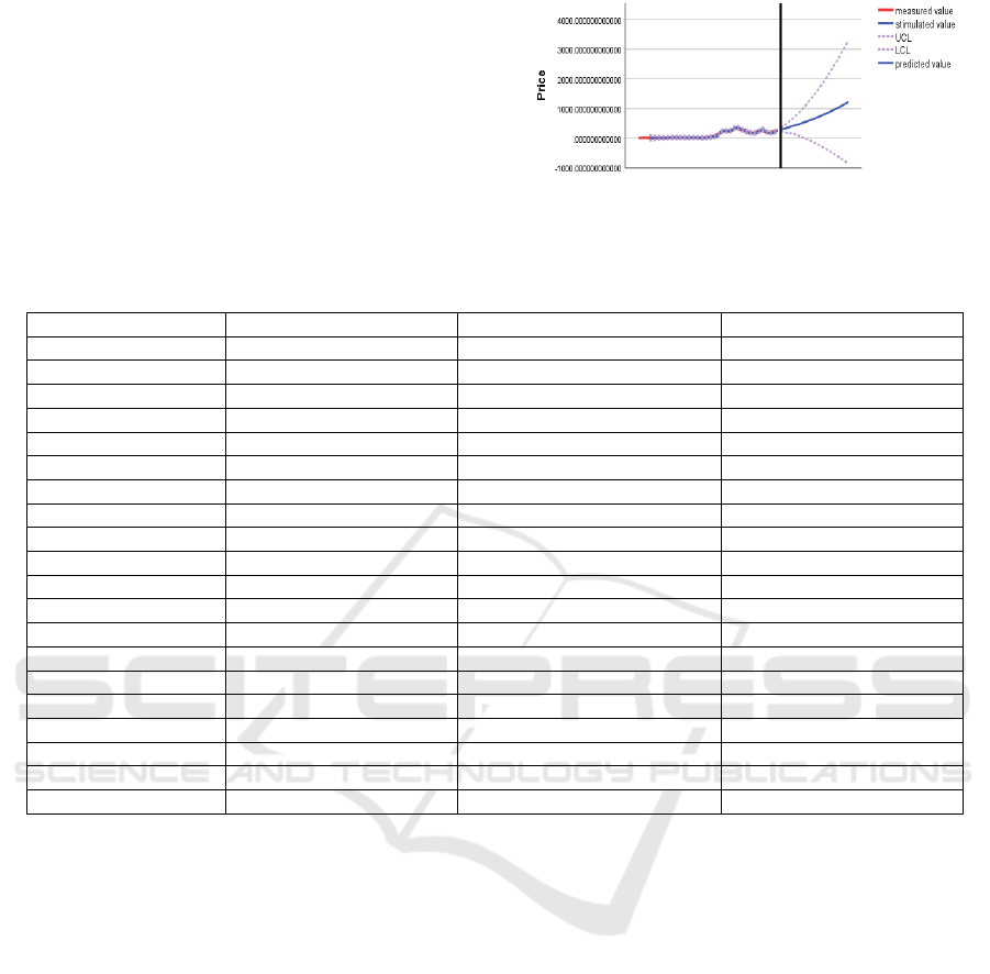
line represents the predicted value. It can be found

from Figure 5 that the stock price will continuously

increase in the next 5 years, and it’s likely to exceed

$1200 by 2029. Table 1 gives the precious data, and

in the middle of the dotted line is the 95% confidence

interval.

Figure 5. Stimulated and predicted stock price change

(Photo/Picture credit: Original).

Table 1: Precious stock price in 2025-2029

Time

(

Quarter, Year

)

Predicted Price

(

)

LCL UCL

Q1 2025 301.6293011 252.1551754 351.1034267

Q2 2025 316.8827521 202.4157752 431.349729

Q3 2025 358.4375646 185.617707 531.2574221

Q4 2025 402.6755892 172.0697723 633.281406

Q1 2026 434.3701642 133.7808203 734.959508

Q2 2026 466.4846821 83.93952173 849.0298426

Q3 2026 508.7668343 39.63987247 977.8937962

Q4 2026 554.2929998 -5.016655248 1113.602655

Q1 2027 597.0201125 -59.24644218 1253.286667

Q2 2027 640.7031468 -119.7397253 1401.146019

Q3 2027 689.1695907 -180.6923511 1559.031533

Q4 2027 740.5238047 -243.3290515 1724.376661

Q1 2028 792.4847462 -310.682308 1895.6518

Q2 2028 846.093745 -381.8911101 2074.0786

Q3 2028 902.8165449 -454.87806 2260.51115

Q4 2028 962.2022246 -529.7567944 2454.161244

Q1 2029 1023.436895 -607.4716683 2654.345459

Q2 2029 1086.805306 -687.7619093 2861.372521

Q3 2029 1152.870225 -769.8349049 3075.575355

Q4 2029 1221.568875 -853.5760946 3296.713844

4 DISSCUSION

The results of the prediction show that the stock price

in the five years is likely to show an upward trend.

Based on this, the reasons for the price increase are as

follows:

1. The continued growth of the electric vehicle

market. With the global emphasis on environmental

protection and sustainable development, the demand

for electric vehicles will continue to increase in the

next five years. Tesla has deep technical

accumulation and brand advantages. Although its

market share fell from 75% in 2022 to nearly 50% in

2024, it still dominated (Patel, 2025).

2. Technological innovation and new product

launch. Musk, the CEO of Tesla, has said that Tesla's

long-term value will rely not only on electric vehicles

but also on its breakthroughs in robotics, such as

Optimus robots and Robotaxi (Joel, 2025). It is

expected that by 2027, the commercialization of

Optimus robots and the comprehensive promotion of

Robotaxi will become Tesla's two major growth

points.

3. Global market expansion. Tesla’s factories in

Shanghai and Berlin not only meet the needs of the

local market but also provide support for exports

(Joel, 2025). In the next five years, Tesla is expected

to diversify and grow revenue by further expanding

its global market share. In addition, its leading

position in artificial intelligence and autonomous

driving technology will also give it an advantage in

global market competition (Joel, 2025).

In future research, researchers can further use the

wavelet analysis method to analyze and predict. First,

the data is an outlier, which is denoised by wavelet

decomposition and reconstruction algorithm. After

the analysis and prediction by the Wavelet-ARIMA

model, the confidence of the prediction results is

compared. The results showed that compared with the

ARIMA prediction model, the Wavelet-ARIMA

IAMPA 2025 - The International Conference on Innovations in Applied Mathematics, Physics, and Astronomy

prediction model has higher confidence (Li & Cheng,

2021).

5 CONCLUSION

This article selects TESLA stock statistics from the

Kaggle website and predicts the future price of Tesla

’s stock by using the data analysis software SPSS

and programming software Python based on the

ARIMA model. The stock price in the five-year

period is likely to show an upward trend. Within a

95% confidence interval, the price will reach around

$63.3 billion in 2026, about 172.4 billion in 2027,

about 245.4 billion in 2028, and about 307.5 billion

in 2029. For the predicted results, the possible

influencing factors are discussed, which include the

EV market, technological innovation, and Global

market expansion. Finally, the next improvement

solution is made to the limitations of the model. Using

the Wavelet-ARIMA hybrid model to predict, which

can more accurately predict time series data

containing small fluctuations.

REFERENCES

Joel. 2025. TSLA price prediction and forecast.

247wallst.com. 2025-01-17, 2025-02-14.

https://247wallst.com/forecasts/2025/01/17/tesla-tsla-

price-prediction-and-forecast/

Le, J. 2015. Research and application of stock price analysis

based on time series. Dalian University of Technology.

Li, Q., Cheng, L. 2021. Time series ARIMA model

prediction method based on wavelet analysis. Journal

of Chenyang Normal University Natural Science

Edition, 39(01), 49–53.

Mao, Y. 2020. Research on combinatorial prediction model

based on time series. Jiangxi University of Finance and

Economics. DOI 10.27175/d.cnki.gjxcu.2020.001417.

Patel, N. 2025. Where will TESLA be in 5 years. fool.com.

2025-01-26, 2025-02-14.

https://www.fool.com/investing/2025/01/26/where-

will-tesla-be-in-5-years/

Wu, D. 2024. Tesla speed is expected to be refreshed.

Liberation Daily, (001).

Xi, L. 2024. Tesla cuts its price at the end of the year mode

Y hits the lowest price in history. Daily Economic News,

2024-12-26(006).

Xiao, Y. 2024. Application of time series prediction.

Statistical Science and Practice, 10, 33–35+43.

Zhang, Y. 2020. Stock price analysis and forecast based on

time series. North China Electric Power University

Beijing. DOI 10.27140/d.cnki.ghbbu.2020.000981.

Zhou, J. 2024. Stock forecast based on ARIMA model -

Taking Bank of China as an example. Modern

Computer, 30(14), 89–92.

Zuo, X. 2019. ADF unit root test with high-order trend

terms. Quantitative Economics and Technological

Economic Research, 36(01), 152–169.

Analysis and Prediction of TESLA Stock Based on the ARIMA Model