Real-Time Fault Detection and Diagnosis for Oil Well Drilling Using a
Multitask Neural Network
Marios Gkionis
1 a
, Ole Morten Aamo
1 b
and Ulf Jakob Flø Aarsnes
2 c
1
Department of Engineering Cybernetics, Norwegian University of Science and Technology, Trondheim, Norway
2
Energy Modelling and Automation, NORCE Energy, Oslo, Norway
Keywords:
Fault Detection, Fault Diagnosis, Deep Neural Networks, Multitask Learning, Oil Well Drilling.
Abstract:
Drilling operations can be unexpectedly laden with mechanical faults, mud loss, and insufficient cuttings
transport that incur substantial costs. This can be avoided via accurate and early fault detection and diagnosis.
We present a novel Drilling Fault Detection and Diagnosis (FDD) system that leverages Multitask Neural
Networks (MTL-NNs). It accounts for the practical limitation that down-hole measurements are normally not
available in real-time and can perform FDD relying only on flow and pressure measurements at the drilling rig.
Data for training and testing are produced by a simulator based on the distributed flow and pressure dynamics
in the entire well governed by four coupled hyperbolic partial differential equations. Faults are incorporated
into the simulations so that the data contain information about how diagnostics of faults affect the dynamics.
Our numerical experiments, admittedly under quite ideal conditions, show that the proposed method exhibits
high generalization performance on diagnosis for fixed well depths, while incorporating varying well depths
into a single network requires increased size in both network and training data to maintain performance.
1 INTRODUCTION
Detection of the presence of a system fault, localiza-
tion and quantification constitute the field of engineer-
ing known as Fault Detection and Diagnosis (FDD).
Numerous techniques have been developed in this
field (Isermann, 2006), and they can be categorized as
data-based or model-based. The former (Venkatasub-
ramanian et al., 2003) utilize historic process knowl-
edge such as datasets from already occurred faults that
can help with detection and prognosis of future faults.
Rich historic datasets for faulty cases in drilling are
absent, since each new well corresponds to a new
(unseen) process. In addition, collecting faulty data
(on purpose) would be an unrealistically expensive
and lengthy process, probably making model-based
methods the more feasible option for FDD in drilling.
A common instance in the list of model-based FDD
methods is the design of a bank of observers (Zhang,
2000), which can be based on Kalman filters, such as
in (Jiang et al., 2020). Separate models are deployed
for incorporation of the individual faults. Each ob-
a
https://orcid.org/0009-0009-2626-9378
b
https://orcid.org/0000-0001-6899-1451
c
https://orcid.org/0000-0001-6272-7203
server corresponds to a model and is designed such
that the process states and outputs are estimated and
predicted respectively. The output prediction errors
(residuals) are stored for statistical change analysis,
thereby providing fault detection and identification.
Methodical design of the statistical change detection
algorithm and the observers is required and a notable
example of this method applied to drilling can be
found in (Willersrud et al., 2015) using down-hole
measurements. However, down-hole measurements
are normally not available in real-time in practice, so
in the present work we rely only on top-side measure-
ments.
Deep Learning (DL) has received rapidly increas-
ing attention from researchers and engineers since
massive amounts of data from processes are collected
and create the opportunity of insight from their sys-
tematic analysis and computational tools have been
improving. The enhancement of the capabilities of
DL has brought about the increase in prediction ac-
curacy, realization of explainability, and savings in
training time and utilization of memory (Alzubaidi
et al., 2021). In addition, two methods that help en-
hance generalization performance and data efficiency
are MTL and Physics-Informed NNs (PINNs) (Raissi
et al., 2019). The latter do so by employing math-
350
Gkionis, M., Aamo, O. M. and Aarsnes, U. J. F.
Real-Time Fault Detection and Diagnosis for Oil Well Drilling Using a Multitask Neural Network.
DOI: 10.5220/0013783800003982
Paper published under CC license (CC BY-NC-ND 4.0)
In Proceedings of the 22nd International Conference on Informatics in Control, Automation and Robotics (ICINCO 2025) - Volume 1, pages 350-361
ISBN: 978-989-758-770-2; ISSN: 2184-2809
Proceedings Copyright © 2025 by SCITEPRESS – Science and Technology Publications, Lda.

ematical models that encode constitutive (physical)
laws (physics priors) that describe the available data,
which are normally either combined with the physics
priors, or the priors can fully replace the data. The
latter option may be desirable in applications such as
drilling, given the absence of historic field data.
MTL-NNs (Caruana, 1997) are NN variants
which are simultaneously trained for multiple sep-
arate prediction tasks, parameterized by shared and
task-specialized parameters. Since it is a Deep Neu-
ral Network (DNN), its utilization does not come
with the requirement of convergence analysis and in-
vestigation of appropriateness as a parameter estima-
tion scheme. This requirement relaxation renders the
implementation quicker and less application-specific.
Up to our knowledge, MTL is at an early stage of in-
corporation on FDD problems. The majority of pub-
lished work focuses on bearings (such as (Guo et al.,
2020), (Liu et al., 2021), and (Wang et al., 2022)) and
wind turbine fault diagnosis.
FDD for Drilling is fundamentally different than
FDD for the aforementioned applications. In Drilling,
faulty data for a new well being drilled are not avail-
able and historical data are not expected to be suf-
ficient for DNN training and Transfer-Learning to a
new well. In rolling bearing FDD, rich operation data
can be utilized to extract accurate fault signatures.
What is more, numerous sensors can be placed in dif-
ferent locations in rotary machinery applications to
extract data, whereas in our case we aim to achieve
FDD only using three time-series signal inputs, one
of which is a manipulated signal. The current work
serves as a starting point for investigating the applica-
tion of MTL for FDD in drilling.
In many applications, data is available from
sources that are described by inter-related latent
mechanisms. Such mechanisms can be encoded
through the shared part of a MTL-NN. To indepen-
dently train individual NNs for each task would lead
to redundant calculations of forward passes of the
shared features and failure to encode the common fea-
tures, thus leading to poorer generalization and pa-
rameter efficiency. The work in (Wang et al., 2021a)
exemplifies this, wherein the rolling bearing vibration
signals are considered in the training of the common
NN, leading to the enrichment of the encoded infor-
mation in the shared features. In general, learning
performance can be improved when auxiliary tasks
are incorporated into the NN, such as with the case
of (Amyar et al., 2020) that uses the COVID classi-
fication task to enhance the learning performance of
the other (main) tasks. MTL can also be valuable
when sensor data are not sufficient for effective Single
Task Learning (STL), as highlighted in (Wang et al.,
2021a). Among the different MTL architectures, we
employ the Multi-Head architecture (MH-NN), which
belong to the Hard-Parameter Sharing class of MTL
architectures (Yu et al., 2024).
It has been stressed in the literature that MH-
NNs are suitable for meta-learning (Hospedales
et al., 2020). For example, the work of (Wang
et al., 2021b) analyzes the connection between meta-
learning and MTL through MH-NNs. In (Zou and
Karniadakis, 2023), successful few-shot learning is
achieved through deployment of MH-NNs, providing
the first empirical observation of synergistic learning.
(Lin et al., 2021) showed that MH-NNs can perform
task-specific adaptation as well. This is a key motiva-
tion for opting to utilize MH-NNs in our pipeline.
In this work, the training data is generated using a
transient drilling hydraulics model described by a sys-
tem of four first order semilinear partial differential
equations (PDEs). Despite the fact that this clearly
encodes the physics of the process into the NN, it
is not strictly a PINN, given that the latter utilizes
the operator terms of the underlying physical laws
in the NN’s loss function (Raissi et al., 2019). It
represents a step further from our work in (Gkionis
et al., 2025), wherein a steady-state model was uti-
lized instead. The MTL-NN approach is similar to
the model-based approach, since each fault requires
a separate model for data generation. Given that the
NN encodes the shared feature representations, fault-
independent observer design is redundant. Moreover,
the NN inherently incorporates and learns the statis-
tical assessment of residuals in the case of the design
bank of observers. We examined three different flow-
related faults, which are detailed at the beginning of
Section 3.
There are a few publications on Drilling FDD that
utilize MTL and PINNs, albeit not referenced in an-
alytical overviews of NN variants and FDD applica-
tions such as (Qiu et al., 2023). For instance, Convo-
lutional NNs are applied in (Jeong et al., 2020) and
(Jan et al., 2022), since the faults are provided as in-
puts in the form of multi-channel time series. How-
ever, these works solely examine Washout Fault De-
tection and up to our knowledge constitute the only
ones that apply PINNs and MTL in Drilling. In (Jan
et al., 2022), the different tasks include a classifica-
tion task and the enforcement of physical constraints.
However, the physics prior used in the estimation is
tied to a specific parametric model, which restricts the
generality of the NN.
We have outlined the rest of this publication as fol-
lows: Section 2 describes the pipeline of the FDD
scheme; the data collection, the formulation of the
data-source, and the structure and loss functions of
Real-Time Fault Detection and Diagnosis for Oil Well Drilling Using a Multitask Neural Network
351

the NN. Section 3 describes the relevant physics of
the application under study and declares which exact
signals are to represent the generic signals defined in
Section 2. We discuss the results in Section 4 and con-
clude with ideas for extending the scope of this work
in Section 5.
2 PROBLEM STATEMENT AND
METHODOLOGY
We consider a construction task that is scheduled to
be set into operation some time in the future. It is
assumed to be unique, so that there is no experi-
enced data available to learn from prior to the op-
eration. However, we assume that the operation can
be described by a dynamic system, taking inputs, de-
noted u : [0, T ] → R
p
, and giving outputs, denoted
y : [0,T ] → R
q
, that we assume will be available as
measurements in real time during the operation. At
any given time, one of m distinct faults may arise, in-
fluencing the relationship between inputs and outputs.
The operation is precisely defined so that a numeri-
cal simulator incorporating the potential faults can be
built and used for planning prior to performing the
operation in practice. Given a sequence of inputs,
{u}
n
i=1
(for some arbitrary n), the type of fault (if
any), an r-dimensional column-vector characterizing
the fault, d ∈ [−1,1]
r
, and an s-dimensional vector of
(physical) system parameters θ ∈ [−1, 1]
s
, the simula-
tor computes the corresponding sequence of outputs,
{y}
n
i=1
. We will denote this simulation as S
i
, where
the index i ∈ {0,1,...,m} identifies the type of fault,
with i = 0 corresponding to the fault-free operation.
In other words, we have
{y}
n
j=1
= S
i
({u}
n
j=1
,d, θ), i ∈ {0,1,...,m}. (1)
θ can represent system parameters that are ex-
pected to change during operation, or whose inclu-
sion in training can elevate the generalization perfor-
mance of the DNN through the mechanism of MTL.
Using data produced by the simulator, we aim to train
a DNN so that it can be used in real time during the
actual operation to detect a fault happening and yield
an alarm with the type of fault and its characteriz-
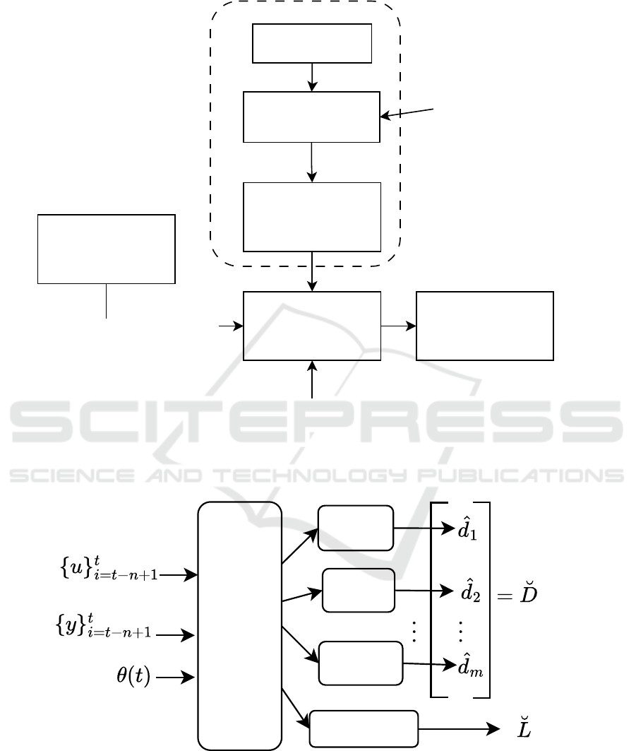
ing vector d. (see Figure 1 for the proposed work
flow). Denoting the neural network as f , we suggest
the input-output structure
(
˘
L,
˘
D) = f ({u}
n
i=1
,{y}
n
i=1
,θ) (2)
where
˘
L ∈ R
m+1
and
˘
D ∈ R
r×(m+1)
. For fault de-
tection, define the one-hot labeling vectors L
i
=
[l
0
,...,l
m
] where l
j
= 1 for j = i and l
j
= 0 for j ̸= i,
and let
ˆ
L equal the L
i
, i ∈ {0,...,m} that is most sim-
ilar to
˘
L. The corresponding estimate of the diagnos-
tics is then given by
ˆ
d =
˘
D
ˆ
L. We suggest Algorithm
1 for generating data for training and testing.
Algorithm 1: Data Generation.
Result: Datasets X and Y filled with
input-output samples
Initialize datasets X and Y as empty;
while number of samples not reached do
Select i randomly from {0,...,m};
Select {u}
n
i=1
randomly from a class of
admissible input signals;
Select d randomly from [−1,1]
r
;
Select θ randomly from [−1,1]
s
;
Compute {y}
n
i=1
= S
i
({u}
n
i=1
,d, θ);
Add {u}
n
i=1
,{y}
n
i=1
,θ to dataset X , and
L
i
,dL
i
to dataset Y ;
end
Let the data sets X,Y produced by Algorithm 1
contain N samples ({u}
n
i=1
,{y}
n
i=1
,θ)
j
, (L
j
,D
j
), j ∈
{1,...,N}. Invoking the NN (2) for each sample in X
produces the predictions
˘
L
j
,
˘
D
j
, j ∈ {1,...,N}. The
loss used for training is
L = L
f d
|{z}
fault detection
+ L
d
|{z}
diagnosis
(3)
where
L
f d
= −
1
N
N
∑
j=1
L
j
· log
˘
L
j
(4)
and
L
d
=
1
N
N
∑
j=1
L
j
W ||(D
j
−
˘
D
j
)L
j
||
2
. (5)
W = [w
0
,w
1
,...,w
m
]
T
is a vector of weights.
In the above, we have for notational simplicity ig-
nored the fact that the diagnostics, d, may have di-
mension less than r for some faults (and dimension 0
for the fault-free case). This is handled in the imple-
mentation by masking out irrelevant components of d
during training and testing.
At every timestep, t, the sequences of inputs,
outputs, and parameters, {u}
t
i=t−n+1
,{y}
t
i=t−n+1
, and
θ(t), from the operation can be fed to the pre-trained
neural net to provide fault detection and diagnostics
in real time, that is
(
˘
L(t),
˘
D(t)) = f ({u}
t
i=t−n+1
,{y}
t
i=t−n+1
,θ(t)) (6)
ˆ
L(t) = argmax
L
i
,i∈{0,...,m}
L
i
· log
˘
L(t) (7)
ˆ
d(t) =
˘
D(t)
ˆ
L(t) (8)
ICINCO 2025 - 22nd International Conference on Informatics in Control, Automation and Robotics
352

Process Planning
Simulator setup
(multiple simulations)
NN Training for FDD
(FDD-NN)
FDD-NN
ALARMS AND
DIAGNOSTICS
Real-Time Data-feed
Real-Time operation
Planning and preparation phase
No available data prior to
plant being built
Meta-learning NN
adaptation in presence of
real-data
Figure 1: Data and process-planning pipeline.
COMMON
TRUNK
head 1
head 2
head m
head m+1
Figure 2: Depiction of a Multi-head Neural Network. Each one of the ”heads” corresponds to a separate Fault with the last
one corresponding to the detection task. Nomenclature of this figure corresponds to equations (6) - (8). The input θ represents
process parameters for which the dataseries are produced. This is an input that is relevant when the training data are produced
by different system parameters.
Real-Time Fault Detection and Diagnosis for Oil Well Drilling Using a Multitask Neural Network
353

This FDD scheme is depicted in Figure 2. The
MTL architectures tested for this work belong to
the Hard Parameter Sharing architecture (Yu et al.,
2024), meaning that the tasks share a subset of pa-
rameters and utilize a subset of specialized parame-
ters which are not shared with the other tasks. Fig-
ure 2 offers a general depiction of such an archi-
tecture. Specifically, we compared the generaliza-
tion performance between two similar architectures:
Fully Connected Multi-task NN (FCN-MTL-NN) and
Multi-head NN (MH-NN). The latter terminology is
not consistent in the literature (Yu et al., 2024). In
this work, we use this terminology when referring to
a NN that uses separate DNNs for each head, whereas
a Fully Connected Multi-task NN the heads are simply
the last activation function of the final linear operation
of the output layer. The consideration of certain pro-
cess parameters θ is important for cases during which
the system parameters change during operation. In-
stead of training multiple separate DNNs, we leverage
the context-sensitive MTL architecture (Silver et al.,
2008) for the system parameters and rely on a larger,
more generalized DNN. In this architecture, a task-
indicator (in this case, the system parameter vector θ)
is propagated in the DNN from the input. In addition,
more context-sensitive parameters may help achieve
a higher generalization performance, which we opt to
leverage in future work.
3 APPLICATION TO DRILLING
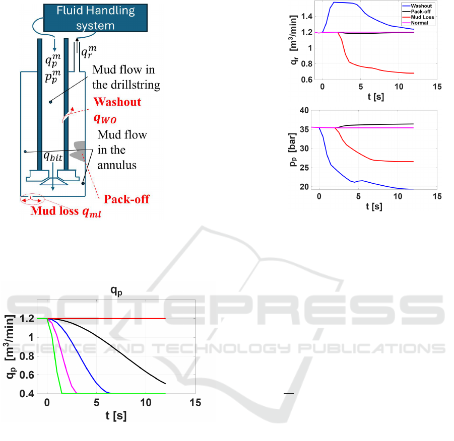
Figure 3a illustrates the drilling process. Measured
quantities are indicated with the superscript m, while
faults are highlighted in red. Drilling fluid, or ”mud,”
is pumped through the drill string to the drill bit and
then returns through the annulus to the Fluid Handling
System (FHS), where it is cleaned and recirculated
into the well. The pump rate q
p
serves as the process
input (u(t) = q
p
(t)), while the pump pressure p
p
and
return flow q
r
are the outputs (y(t) = [p
p
(t),q
r
(t)]).
The relationship between input and output varies de-
pending on whether a fault is present. The FHS is
assumed to be open to the atmosphere on the annu-
lus side, meaning that the pressure at that boundary is
fixed at 1 bar. Managed Pressure Drilling (MPD) can
be easily integrated as long as the pressure at the inlet
of the MPD choke and the flow rate of the backpres-
sure pump are measured. Washout occurs when fluid
bypasses the normal flow path due to a crack or hole in
the drill string, causing a shortcut from the drill string
to the annulus. Its diagnostics include the crack loca-
tion and size, represented as z
wo
and C
wo
. Mud loss
happens when drilling fluid leaks from the well into
Table 1: Training parameters.
Parameter Value
Batch type Mini batch (size=400)
Number of sam-
pled trajectories
{Washout: 8000, Packoff:
8000, Mud loss: 8000}
Layer structure
for head
NN
head
=
[80,80,80, 80, 80, 80,2]
MH-NN struc-
ture
[75, 1699, 1699, 1699,
NN
head
, NN
head
, NN
head
,
[80, 80, 80, 80, 80, 80, 4]]
FC-NN struc-
ture
[75, 1272, 1272, 1272,
1272, 1272, 12]
Number of
trainable pa-
rameters
MH-NN: 6580134, FC-NN:
6588972
Activation func-
tions
GELU (and SoftMax for the
categorization output)
Loss function Diagnosis: MSE, Detection:
Cross Entropy
Regularization L2 (0.01)
Optimizer AdamW (0.9,0.9)
(Loshchilov and Hutter,
2017)
Hardware NVIDIA RTX A2000 Lap-
top GPU (cuda) with Py-
Torch
the reservoir. The key diagnostics for mud loss are
the reservoir pressure and the mud-loss coefficient,
denoted as p
r
and k
I
respectively. Pack-off refers to
the partial or complete blockage of recirculation flow,
often caused by inadequate hole cleaning, which al-
lows cuttings to accumulate in the well. The key di-
agnostic for pack-off is the size coefficient linked to
the pressure-drop across the blockage denoted by C
po
.
See equations (10) - (12) in the Appendix for details
of the fault modeling.
The task of constructing an oil well constitutes a
unique operation of the sort introduced in Section 2.
The well is planned in detail before the operation, fa-
cilitating the setup of a simulator of the operation.
In this work, we base the simulator on a mathemat-
ical description of the pressure and flow in the drill
string and annulus in the form of a hyperbolic par-
tial differential equation. The details of the model
are given in the Appendix. For a constant pump rate
of q
p
(t) = 1200 [l/min], Figure 3b shows the return
flow and pump pressure computed by the simulator
for carefully selected examples of the three faults of
interest. Notice that the pump pressure and return rate
stay constant in the fault-free case (magenta lines).
In the case of washout (blue lines), the return rate
suddenly increases due to the short-cut suddenly cre-
ated by the crack in the pipe. It quickly returns to
ICINCO 2025 - 22nd International Conference on Informatics in Control, Automation and Robotics
354

(a) Well schematic, depicting the Faults consid-
ered for this work. Figure from (Gkionis et al.,
2025).
(b) Simulated trajectories from the Partial Differ-
ential Equations describing the system (see Ap-
pendix), showcasing the different behavior in-
duced by the occurrence of different Faults.
Figure 3: Well schematic (left) and signatures of the different Faults (right).
Figure 4: Different q
p
trajectories. Each different color cor-
responds to a different set of A and γ of Equation (9). Blue:
[0.8, 0.47], black: [0.8, 0.2], red: [0.8, 0], purple: [0.8, 1],
green: [0.8, 02].
the original value of the pump flow, though, as mass
balance is enforced. Due to the short-cut, the flow
experiences less frictional pressure loss, and the re-
quired pump pressure to circulate therefore decreases.
In the case of mud loss (red lines), the return flow
decreases and stays low because mud is permanently
lost to the reservoir. Less fluid therefore circulates,
requiring a lower pump pressure. In the pack-off case
(black lines), the flow stays relatively constant (since
no mud is lost), while the frictional pressure loss in-
creases due to the restriction pack-off causes, requir-
ing a higher pump pressure to circulate. The pressure
and flow signatures of the faults show quite distinct
features that can easily be identified by visual inspec-
tion. The purpose of the neural network, however, is
to detect as early as possible less obvious faults that
may evolve into serious problems for the operation if
not counteracted.
Data for training and testing is produced accord-
ing to Algorithm 1. In the algorithm, a set to draw
admissible input signals from is defined by
q
p
(t) =
A
j
2

cos

max

0,min{γ
j
t,π}

+ 1

(9)
where the parameters A
j
,γ
j
are uniformly sampled
from [0.2,1.0] and [0,2π/T
lim
] respectively. This cor-
responds to ramping the pump down from a rate gov-
erned by A
j
at a slope governed by γ
j
, which are likely
operations of the pump in practice. Examples of this
are shown in Figure 4.
As it has been already mentioned, this work
focuses on performing accurate Diagnosis in the
Drilling application. It is assumed that the faults do
not occur simultaneously and that the system is oper-
ating in steady-state up until a fault occurrence.
As a first step to assessing the robustness of the
FDD scheme, we generate data using simulations for
uniformly sampled values of the depth of the well L
in the range [2000m,4000m]. The architecture used
for this addition is the one shown in Figure 2 with
θ(t) equal to L(t) normalized to the interval [−1,1].
L clearly varies slowly compared to the dynamics of
pressure and flow.
Real-Time Fault Detection and Diagnosis for Oil Well Drilling Using a Multitask Neural Network
355

Table 2: Detection accuracy for the different faults.
- Washout Mud Loss Pack-off
Fixed depth (3000m) 99.5% 100% 100%
Variable depth 99.7% 100% 100%
The motivation for using the specific time window
of T = 12s and sampling time of ∆t = 0.5s is linked
to the dynamics of the system. The nature of the pres-
sure waves in this system is such that there will be a
delay until the effects of a fault become apparent at
the topside boundary. This can be verified via visual
inspection of the delays for the first signal changes to
occur Figure 3b).
4 RESULTS AND DISCUSSION
The hyperparameters of the training algorithm are
provided in Table 1. Figures 5a and 5b show the scat-
terplots for the predictions on the diagnostic variables
for fixed (first row) and randomized well depth (sec-
ond row) for Washout and Mud Loss respectively and
Figure 6 shows the same information for Pack-off. In
this section, we present the results of applying the test
data to the trained network. The performance of clas-
sification of the type of fault (i.e. fault detection) is
summarized in Table 2 for the cases of fixed and vari-
able well depth. It can be observed that Diagnosis
is accurate when the well depth is fixed and exhibits
moderate robustness with respect to the well depth
parameter. The MH-NN trained on data a fixed well
depth of 3000 m exhibits quite higher accuracy using
the same number of training datapoints (8000).
1. The MH-NN (Figure 2) generalizes equally well
with a FCN that has multiple outputs. The depth
of the NN was crucial to the results; a shallow NN
(with the same number of trainable parameters)
resulted in gradient vanishing , as well as with
depth quite larger than the one used for this work.
2. The NN trained for trajectories with randomly
sampled well depths exhibited unsurprisingly
lower accuracy for Fault Diagnosis. Enlarging
the training dataset and/or the NN would improve
the prediction accuracy. In addition, utilization of
useful biases linked to the effect of the well depth
in the dynamics, and application of meta-learning
in already trained NNs can result in improvement
of the NN’s generalization performance.
3. The outliers in Figure 5a and Figure 5b are not
surprising. C
wo
becomes difficult to correctly di-
agnose when the washout occurs close to the bit,
since then the flow through the crack and the
flow through the bit are indistinguishable from
the top-side, several kilometers away. Diagnosing
z
wo
for small washouts is also quite difficult be-
cause accurate localization is sensitive to the dif-
ference between the pump rate and the rate of flow
through the bit. It is this difference that causes
a change in the pump pressure which can be de-
tected top-side. When it comes to mud loss (Fig-
ure 5b, the reservoir pressure p
r
is generally well
predicted, while the index k
I
is occasionally quite
wrong. We do not have a clear explanation for
this behavior, but in practice, it is more impor-
tant to obtain an accurate estimate of the reservoir
pressure because then the down-hole pressure one
needs to aim for in order to stop the loss is known.
The down-hole pressure can be lowered to some
extent by ramping down the pump, and to a larger
extent by changing the mud weight.
4. The high prediction quality (for fixed well depth),
achieved without weight scheduling or special
regularization (Mao et al., 2024), suggests that
task domination (Senushkin et al., 2023) may be
absent in the studied datasets.
5. In spite of the established theory (Zhang et al.,
2016) that overparameterization generates im-
plicit regularization, the multi-head architecture
still required weight decay in order to generalize
in an acceptable level.
5 CONCLUSIONS AND FUTURE
WORK
In this work, a MTL-NN was successfully trained
to perform accurate Fault Diagnosis through deploy-
ment of a single multi-head NN trained on simulated
time-series trajectories. It constitutes a preliminary
step towards using generalized NNs that predict ac-
curately for wider spectrum of faults and well param-
eters, as well as parameters of the fault-free process.
Our NN generalizes to different well depths with sig-
nificant room for improvement. In addition, the re-
quirement for an increased network depth is typically
suggestive of the presence of hierarchical complexity
in the dataset.
An immediate idea for extending this work would
be to improve the data-efficiency of MTL that per-
ICINCO 2025 - 22nd International Conference on Informatics in Control, Automation and Robotics
356

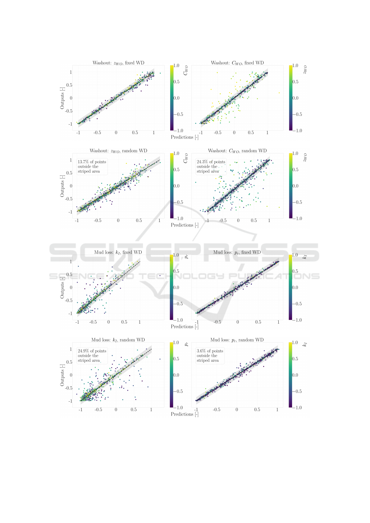
(a) Scatterplots of Washout diagnostics on test data, using the MH-NN for fixed Well Depth and random Well
Depth
(b) Scatterplots of Mud Loss diagnostics on test data, using the MH-NN for fixed Well Depth and random Well
Depth
Figure 5: Scatterplots for the faults. The values are normalized in [-1, 1]. The x-axis represents the network’s prediction and
the y-axis represents the actual values for the diagnostics.
Real-Time Fault Detection and Diagnosis for Oil Well Drilling Using a Multitask Neural Network
357

(a) Scatterplot of Pack-off diagnostics on test data, using the
MH-NN.
(b) Scatterplot using MH-NN trained on randomized well
depth data.
Figure 6: Scatterplots for the faults. Values normalized in [−1, 1]. The x-axis represents the network’s prediction and the
y-axis represents the actual values for the diagnostics.
forms FDD with the same NN for different well
depths (as well as other well characteristics, such as
the well geometry, varying drill string cross-sections,
and drilling fluid), given the satisfactory accuracy that
we have achieved using the same NN that was trained
for data generated using a fixed well depth.
In addition to this, considering more well param-
eters would bring about higher generalization per-
formance and creating a more general NN that can
then be used to finely update a subset of the Network
parameters for unseen wells based on meta-learning
(Hospedales et al., 2020) and few-shot learning (Zou
and Karniadakis, 2023). What is more, it is specu-
lated that the consideration of multiple sources of pa-
rameter uncertainty will render detection of the faults
challenging, since it is expected that there will be very
similar curves corresponding to different faults and
different well parameters. This possibility gives rise
to the requirement for developing and training NNs
that incorporate uncertainty (He and Jiang, 2023).
Further work on rendering the scheme more robust
and realistic via incorporating uncertainty in the data
and the system parameters would be to include col-
ored noise in the input data.
The most important limitation of our work is, ad-
mittedly, the complete reliance on simulated data for
NN training. The motivations for this are as follows.
• Preliminary investigation of the feasibility of per-
forming FDD given the known dynamics of a
problem. Up to our knowledge, this is the first
work that tackles the inverse problem of identify-
ing fault parameters in drilling for multiple faults
and utilizing only topside measurements. There-
fore, a first step towards FDD is to investigate its
feasibilty with synthetic data.
• Insufficient number of real process data. As ex-
plained in Section 1, real drilling data during
faulty operations are not expected to be sufficient
for DNN training. This is true for other applica-
tions as well (for example, in (Tercan et al., 2018)
and (Weber et al., 2020)). Tackling this chal-
lenge requires utilization of methods that transfer
knowledge from simulations to real data.
Since the synthetic data bear similarities with the
real drilling data, the knowledge encoded in DNNs
trained with simulation data may be exploited such
that the DNN adapts to sparse real process data. The
techniques that facilitate this adaptation are Trans-
fer Learning and Meta-Learning (Hospedales et al.,
2020), (Ranaweera and Mahmoud, 2021). Numer-
ous industrial applications which leverage Transfer
Learning exist in literature, many of which are de-
tailed in (Yan et al., 2023). For example, the au-
thors in (Tercan et al., 2018) tackle the problem of low
availability of real industrial data for training in injec-
tion mold methods by training a DNN with simulated
data and then introduce new NN parameters for train-
ing on real data while keeping the simulation-trained
ones frozen, or use the already trained values of the
weights as initial values for training with the limited
real training data. The authors in (Weber et al., 2020)
train base DNN models to detect room occupancy us-
ing synthetic data from room occupancy simulations
and physical simulations. These base models are sub-
sequently updated through a transfer step to adapt to
the limited (and more expensive to sample) real data.
Up to our knowledge, there is not any research work
that applies Transfer Learning and/or Meta-Learning
to bridge the gap between simulated and real data in
drilling applications.
Last but not least, to enhance the practicability of
the developed algorithm, extensive testing with state-
ICINCO 2025 - 22nd International Conference on Informatics in Control, Automation and Robotics
358

of-the-art drilling simulators can be conducted. Such
simulators (for example, OpenLAB from (Gravdal
et al., 2021)) can model faults which cannot are gov-
erned by much more complicated dynamics, such as
Gas-Kick (Sun et al., 2018).
REFERENCES
Alzubaidi, L., Zhang, J., Humaidi, A. J., Al-dujaili, A.,
Duan, Y., Al-Shamma, O., Santamar
´
ıa, J. I., Fadhel,
M. A., Al-Amidie, M., and Farhan, L. (2021). Review
of deep learning: concepts, cnn architectures, chal-
lenges, applications, future directions. Journal of Big
Data, 8.
Amyar, A., Modzelewski, R., and Ruan, S. (2020). Multi-
task deep learning based ct imaging analysis for
covid-19: Classification and segmentation. medRxiv.
Caruana, R. (1997). Multitask learning. Machine Learning,
28:41–75.
Gkionis, M., Wilhelmsen, N. C. A., and Aamo, O. M.
(2025). Fault diagnosis for drilling using a multitask
physics-informed neural network. In Proceedings of
the 14th IFAC Symposium on Dynamics and Control
of Process Systems, including Biosystems (DYCOPS).
To appear.
Gravdal, J. E., Sui, D., Nagy, A. P., Saadallah, N., and
Ewald, R. (2021). A hybrid test environment for veri-
fication of drilling automation systems.
Guo, S., Zhang, B., Yang, T., Lyu, D., and Gao, W. (2020).
Multitask convolutional neural network with informa-
tion fusion for bearing fault diagnosis and localiza-
tion. IEEE Trans. Ind. Electron., 67(9):8005–8015.
He, W. and Jiang, Z. (2023). A survey on uncertainty quan-
tification methods for deep learning.
Hospedales, T. M., Antoniou, A., Micaelli, P., and Storkey,
A. J. (2020). Meta-learning in neural networks: A
survey. IEEE Transactions on Pattern Analysis and
Machine Intelligence, 44:5149–5169.
Isermann, R. (2006). Fault-diagnosis systems : an introduc-
tion from fault detection to fault tolerance.
Jan, A., Mahfoudh, F., Dra
ˇ
skovic, G., Jeong, C., and Yu,
Y. (2022). Multitasking physics-informed neural net-
work for drillstring washout detection. 2022(1).
Jeong, C., Yu, Y., Mansour, D., Vesslinov, V., and Meehan,
R. (2020). A physics model embedded hybrid deep
neural network for drillstring washout detection.
Jiang, H., hui Liu, G., Li, J., Zhang, T., and Wang,
C. (2020). A realtime drilling risks monitoring
method integrating wellbore hydraulics model and
streaming-data-driven model parameter inversion al-
gorithm. Journal of Natural Gas Science and Engi-
neering, page 103702.
Lin, Z., Zhao, Z., Zhang, Z., Baoxing, H., and Yuan, J.
(2021). To learn effective features: Understanding the
task-specific adaptation of {maml}.
Liu, Z., Wang, H., Liu, J., Qin, Y., and Peng, D. (2021).
Multitask learning based on lightweight 1DCNN for
fault diagnosis of wheelset bearings. IEEE Trans. In-
strum. Meas., 70:1–11.
Loshchilov, I. and Hutter, F. (2017). Decoupled weight
decay regularization. In International Conference on
Learning Representations.
Mao, D., Chen, Y., Wu, Y., Gilles, M., and Wong, A. (2024).
Robust analysis of multi-task learning efficiency: New
benchmarks on light-weighed backbones and effective
measurement of multi-task learning challenges by fea-
ture disentanglement.
Qiu, S., Cui, X., Ping, Z., Shan, N., Li, Z., Bao, X., and Xu,
X. Y. (2023). Deep learning techniques in intelligent
fault diagnosis and prognosis for industrial systems:
A review. Sensors (Basel, Switzerland), 23.
Raissi, M., Perdikaris, P., and Karniadakis, G. E. (2019).
Physics-informed neural networks: A deep learning
framework for solving forward and inverse problems
involving nonlinear partial differential equations. J.
Comput. Phys., 378:686–707.
Ranaweera, M. and Mahmoud, Q. H. (2021). Virtual to real-
world transfer learning: A systematic review. Elec-
tronics.
Senushkin, D., Patakin, N., Kuznetsov, A., and Konushin,
A. (2023). Independent component alignment for
multi-task learning. 2023 IEEE/CVF Conference on
Computer Vision and Pattern Recognition (CVPR),
pages 20083–20093.
Silver, D. L., Poirier, R., and Currie, D. (2008). Inductive
transfer with context-sensitive neural networks. Ma-
chine Learning, 73:313–336.
Sun, X., Sun, B., Zhang, S., Wang, Z., Gao, Y., and Li, H.
(2018). A new pattern recognition model for gas kick
diagnosis in deepwater drilling. Journal of Petroleum
Science and Engineering.
Tercan, H., Guajardo, A., Heinisch, J., Thiele, T., Hop-
mann, C., and Meisen, T. (2018). Transfer-learning:
Bridging the gap between real and simulation data
for machine learning in injection molding. Procedia
CIRP, 72:185–190.
Venkatasubramanian, V., Rengaswamy, R., Kavuri, S. N.,
and Yin, K. K. (2003). A review of process fault de-
tection and diagnosis: Part iii: Process history based
methods. Comput. Chem. Eng., 27:327–346.
Wang, H., Liu, Z., Peng, D., Yang, M., and Qin, Y. (2021a).
Feature-level attention-guided multitask cnn for fault
diagnosis and working conditions identification of
rolling bearing. IEEE Trans. Neural Netw. Learn. Syst.
Wang, H., Liu, Z., Peng, D., Yang, M., and Qin, Y.
(2022). Feature-level attention-guided multitask CNN
for fault diagnosis and working conditions identifi-
cation of rolling bearing. IEEE Trans. Neural Netw.
Learn. Syst., 33(9):4757–4769.
Wang, H., Zhao, H., and Li, B. (2021b). Bridging multi-task
learning and meta-learning: Towards efficient training
and effective adaptation. ArXiv, abs/2106.09017.
Weber, M., Doblander, C., and Mandl, P. (2020). Towards
the detection of building occupancy with synthetic en-
vironmental data. ArXiv, abs/2010.04209.
Willersrud, A., Blanke, M., Imsland, L. S., and Pavlov,
A. K. (2015). Fault diagnosis of downhole drilling in-
Real-Time Fault Detection and Diagnosis for Oil Well Drilling Using a Multitask Neural Network
359

cidents using adaptive observers and statistical change
detection. Journal of Process Control, 30:90–103.
Yan, P., Abdulkadir, A., Luley, P.-P., Rosenthal, M., Schatte,
G. A., Grewe, B. F., and Stadelmann, T. (2023). A
comprehensive survey of deep transfer learning for
anomaly detection in industrial time series: Methods,
applications, and directions. IEEE Access, 12:3768–
3789.
Yu, J., Dai, Y., Liu, X., Huang, J., Shen, Y., Zhang, K.,
Zhou, R., Adhikarla, E., Ye, W., Liu, Y., Kong, Z.,
Zhang, K., Yin, Y., Namboodiri, V., Davison, B. D.,
Moore, J. H., and Chen, Y. (2024). Unleashing the
power of multi-task learning: A comprehensive sur-
vey spanning traditional, deep, and pretrained founda-
tion model eras. ArXiv, abs/2404.18961.
Zhang, C., Bengio, S., Hardt, M., Recht, B., and Vinyals,
O. (2016). Understanding deep learning requires re-
thinking generalization. ArXiv, abs/1611.03530.
Zhang, Q. (2000). A new residual generation and evalu-
ation method for detection and isolation of faults in
non-linear systems. International Journal of Adaptive
Control and Signal Processing, 14:759–773.
Zou, Z. and Karniadakis, G. E. (2023). L-hydra: Multi-
head physics-informed neural networks. ArXiv,
abs/2301.02152.
APPENDIX
In this section, the partial differential equations de-
scribing the drilling dynamics, including the poten-
tial faults, are given. The state variables are pressure
in the drill string (p
d
(z,t)), pressure in the annulus
(p
a
(z,t)), volumetric flow in the drill string (q
d
(z,t)),
and volumetric flow in the annulus (q
a
(z,t)). q
p
(t)
is the applied pump rate (volumetric flow) into the
drill string, while p
0
is the atmospheric pressure at
the outlet of the annulus. The well length is L, so that
z ∈ [0,L] and z = 0 is at the top of the well. For sim-
plicity, a vertical well with spatially invariant cross
section is assumed.
The nomenclature with the respective values is
given in Table 3 used in the simulations of Section 3.
The three faults that we consider are modeled as
follows. The washout flow is given by
q
wo
(t) = C
wo
p
p
d
(z
wo
,t) − p
a
(z
wo
,t), (10)
the mud loss flow is given by
q
ml
(t) = k
I
(p
a
(L,t) − p
r
), (11)
and the pack-off pressure loss is given by
p
po
(t) =
A
a
C
2
po
q
2
a
(L,t). (12)
We have opted to diagnose Pack-off by considering
that it takes place at the bottom of the well.
Denoting ∂
x
y ≜
∂y
∂x
and the Dirac delta function by
δ(z), we have the dynamics
∂
t
p
d
(z,t) = −
β
A
d
(∂
z
q
d
(z,t) + δ(z − z
wo
)q
wo
) (13)
∂
t
q
d
(z,t) = −
A
d
ρ
∂
z
p
d
(z,t) − f
d
(q
d
(z,t)) + A
d
g
(14)
∂
t
p
a
(z,t) = −
β
A
a
(∂
z
q
a
(z,t) − δ(z − z
wo
)q
wo
) (15)
∂
t
q
a
(z,t) = −
A
a
ρ
∂
z
p
a
(z,t) − f
a
(q
a
(z,t)) + A
a
g
(16)
+ δ(z − L)p
po
with boundary conditions
q
d
(0,t) = q
p
(t) (17)
p
a
(0,t) = p
0
(18)
p
d
(L,t) = p
a
(L,t) +
1
C
2
bit
q
2
d
(L,t) (19)
q
a
(L,t) = −q
d
(L,t) + k
I
max{p
a
(L,t) − p
r
,0}.
(20)
In practice, only the pump rate q
p
(t), pump pressure
p
p
(t) = p
d
(0,t) and return flow q
r
(t) = −q
a
(0,t) are
commonly measured. The diagnostics are normal-
ized to the interval [−1, 1]. For example, let C
wo
∈
[C
wo,min
,C
wo,max
]. Then, the normalized diagnostic is
given by
d = 2
C
wo
−C
wo,min
C
wo,max
−C
wo,min
− 1. (21)
The simulator implements the dynamics using first or-
der finite differences on a staggered grid.
From Table 3, the friction coefficient quantifies
the pressure drop along a pipe (drillstring and an-
nulus in our case) per unit length for a fluid flow of
1 m
3
/min across the pipe. The formula is given be-
low.
f
d/a
≜ ∆p
d/a
A
d/a
ρ
(22)
∆p
d/a
was selected as 5 bar/km/(m
3
/min)
2
for the
drillstring and 3 bar/km/(m
3
/min)
2
for the annulus.
The bit valve coefficient expresses the pressure
drop over the bit at a given flow. We assumed a 10 bar
pressure drop at 1.5 m
3
/min flow. The valve coeffi-
cient formula is given below.
C
bit
≜
q
p
∆p
bit
/ρ
(23)
ICINCO 2025 - 22nd International Conference on Informatics in Control, Automation and Robotics
360

Table 3: List of symbols in the PDE equations with their respective values (if they correspond to a fixed parameter).
Symbol Description Value
β Bulk modulus of the drilling fluid 1.8 × 10
4
bar
ρ Density of the drilling fluid 1000 kg/m
3
g Acceleration of gravity 9.81 m/s
2
A
d/a
Cross-sectional area of drill
string/annulus
[127,366] cm
2
f
d/a
Drillstring and annulus friction
coefficients
[13.7,65.9] 1/m
3
C
bit
Bit valve coefficient 0.0053 m
3
/s/bar
0.5
C
wo
Washout size coefficient (diagnostic) –
z
wo
Washout location (diagnostic) –
C
po
Pack-off size coefficient (diagnostic) –
z
po
Pack-off location (diagnostic) –
k
I
Flow coefficient for mud-loss
(diagnostic)
–
p
r
Reservoir pressure (diagnostic) –
Real-Time Fault Detection and Diagnosis for Oil Well Drilling Using a Multitask Neural Network
361