Recursive Gaussian Process Regression with Integrated Monotonicity

Assumptions for Control Applications

Ricus Husmann

, Sven Weishaupt

and Harald Aschemann

Chair of Mechatronics, University of Rostock, Rostock, Germany

Keywords:

Machine Learning in Control Applications.

Abstract:

In this paper, we present an extension to the recursive Gaussian Process (RGP) regression that enables the

satisfaction of inequality constraints and is well suited for a real-time execution in control applications. The

soft inequality constraints are integrated by introducing an additional extended Kalman Filter (EKF) update

step using pseudo-measurements. The sequential formulation of the algorithm and several developed heuris-

tics ensure both the performance and a low computational effort of the algorithm. A special focus lies on an

efﬁcient consideration of monotonicity assumptions for GPs in the form of inequality constraints. The algo-

rithm is statistically validated in simulations, where the possible advantages in comparison with the standard

RGP algorithm become obvious. The paper is concluded with a successful experimental validation of the

developed algorithm for the monotonicity-preserving learning of heat transfer values for the control of a vapor

compression cycle evaporator, leveraging a previously published partial input output linearization (IOL).

1 INTRODUCTION

A lot of progress can be noticed regarding the online

identiﬁcation of system models. An example for a

basic method is given by the deﬁnition of paramet-

ric functions like polynomial ansatz functions and the

subsequent use of a recursive least-squares regres-

sion as described in (Blum, 1957). If models with

non-measurable states or parameters are to be identi-

ﬁed, this method can be extended to linear Kalman

Filters (KF) or Unscented/Extended Kalman Filters

(UKF/EKF) as proposed in (Kalman, 1960), (Julier

and Uhlmann, 1997). In the presence of additional in-

equality constraints, especially Moving Horizon Esti-

mation (MHE) techniques are suitable (Haseltine and

Rawlings, 2005). If a more general approach is envis-

aged, there exist online-capable training methods of

neural networks as discussed in (Jain et al., 2014).

Gaussian Processes (GP) have been established

as a popular non-parametric alternative to neural net-

works (NNs). They are usually more data-efﬁcient

than neural networks, robust to overﬁtting and – as

main advantage in comparison to NNs – provide an

uncertainty quantiﬁcation for the predicted value, see

https://orcid.org/0009-0006-0480-8877

https://orcid.org/0009-0007-0601-4605

https://orcid.org/0000-0001-7789-5699

(Sch

urch et al., 2020). The non-parametric character

and the O(n

) rise of computational load in depen-

dency of the utilized data points, however, poses a big

challenge for their online implementation. Neverthe-

less, the literature offers suitable methods to address

this problem, like active-set methods as described in

(Qui

nonero-Candela and Rasmussen, 2005), which

limit the number of utilized measurement points. Fur-

thermore, a promising algorithm was presented by

(Huber, 2013) with the recursive Gaussian Process re-

gression (RGP). The idea here is to deﬁne the GPs as

parametric functions based on user-deﬁned basis vec-

tors. This preserves many beneﬁts of the GP regres-

sion while maintaining a small computational load.

For many modeling tasks, a certain previous

knowledge is available. This may include bounds

on model outputs or monotonicity assumptions. This

knowledge might come from physical properties or

in the form of stability-conserving constraints in a

control setting. Nevertheless, the application of this

knowledge during learning has the potential to pro-

vide superior models with far less data. In neural

networks, such assumptions might be considered by

an altering of the reward function as in (Desai et al.,

2021). For standard GPs, a number of methods are

available for considering assumptions, e.g. regarding

the system structure as presented in (Beckers et al.,

2022) or for inequality constraints as shown in (Veiga

340

Husmann, R., Weishaupt, S. and Aschemann, H.

Recursive Gaussian Process Regression with Integrated Monotonicity Assumptions for Control Applications.

DOI: 10.5220/0013783100003982

Paper published under CC license (CC BY-NC-ND 4.0)

In Proceedings of the 22nd International Conference on Informatics in Control, Automation and Robotics (ICINCO 2025) - Volume 1, pages 340-349

ISBN: 978-989-758-770-2; ISSN: 2184-2809

and Marrel, 2020). To the best of our knowledge,

however, the integration of inequality constraints for

recursive GPs represents a new development.

In (Husmann et al., 2024b), a partial IOL for Va-

por Compression Cycle (VCC) Control including an

integral feedback regarding the heat transfer value

was presented. As mentioned in that paper, the usage

of the steady state of the integrator to derive a data-

based model seems a promising idea. Since mono-

tonicity assumptions hold for the input dependencies

of such a heat transfer value model, this application

represents an interesting candidate for the validation

of the RGP algorithm with the inclusion of mono-

tonicity assumptions.

The main contributions of the paper are:

• Computationally efﬁcient consideration of in-

equality constraints w.r.t. Gaussian variables in

a sequential EKF update

• Integrating monotonicity assumptions into RGP

regression by means of inequality constraints

• Real-time implementation of the presented

online-learning algorithm regarding a data driven

RGP model for the heat-transfer value of a VCC

The paper is structured as follows: First, we re-

capitulate the RGP in Sec. 2. Then, the generalized

approach for considering inequality constraints is pre-

sented in Subsec. 3.1. Afterwards, we introduce the

special case of formulating GP monotonicity as such

a constraint in Subsec. 3.4, summarize and discuss the

complete algorithm. As a ﬁrst validation in Sec. 4, we

statistically analyze the validity of the algorithm for a

simulation example. Finally, an experimental valida-

tion is provided in Sec. 5 with an implementation of

the real-time algorithm on a VCC test rig. The paper

ﬁnishes with a conclusion and an outlook.

2 RECURSIVE GAUSSIAN

PROCESS REGRESSION

In this chapter, we brieﬂy describe recursive Gaus-

sian Process regression (RGP) as presented in (Hu-

ber, 2013) and extended in (Huber, 2014). As usual,

we utilize a Squared Exponential (SE) kernel

k(x

x, x

′

) = σ

· exp(−(x

x − x

′

)

x − x

′

)(2L)

−1

) (1)

with a zero mean function m(X

X) = 0. In our applica-

tion, the hyperparameters L and σ

are user-deﬁned.

As elaborated in Subsec. 2.1, a joint length scale L

is deﬁned for all input dimensions, and the possibly

different input ranges are addressed by an extra nor-

malization step. For each GP, we consider only one

measurement y

per time step k, with a corresponding

measurement variance σ

. As detailed in Subsec. 2.1,

X refers to the constant basis vectors, which are de-

ﬁned during initialization, and X

denotes the current

test input. The mean values µ

and the covariance ma-

trix C

of the kernels, which are updated recursively,

give the RGP algorithm a KF-like structure.

The following variables can be precalculated of-

ﬂine:

Ofﬂine

K = k(X

X,X

X), (2)

= K

−1

= 0

0 ,

= K

K .

Given a zero mean function and a single measurement

per time step, the inference step simpliﬁes to:

Inference

= k(X

, X

X)· K

, (3)

= J

· µ



:

k(X

, X

) + J

− K

K)J

where the superscript p indicates the GP prediction

for the test inputs X

. This prediction is used in the

following update step:

Update

= C

· (C

+ σ

)

−1

, (4)

k+1

= µ

+ G

· (y

− µ

k+1

= C

− G

2.1 Input Normalization

We deﬁne the basis vectors for all input axes as an

equidistant grid with step size 1. This leads to a



∏

i=1



× n

-dimensional matrix which contains

all vertices of the grid, where n

denotes the input

dimension of the GP, and N

the number of points in

the respective dimension. An example for the basis

vectors for n

= 2 , N

= 2 and N

= 3 is

X =







0 1 0 1 0 1

0 0 1 1 2 2



. (5)

To consider the ranges of the actual inputs ζ

in each

dimension, we introduce the normalization step

i,k

= f

norm

(ζ

k,i

) = (ζ

i,k

− ζ

) ·

− 1

− ζ

| {z }

, (6)

which is applied before each GP evaluation. Here

and ζ

denote the corresponding lower and upper

bounds of the input, and β

is a constant factor, which

is used in Subsec. 3.4.

The normalization and the use of a joint length L

was originally introduced to handle numerical issues

Recursive Gaussian Process Regression with Integrated Monotonicity Assumptions for Control Applications

341

that may occur for large L in the standard inversion-

based RGP formulation applied in this paper. With the

normalization step, a universal maximum L

max

– inde-

pendent of the system – can be determined to main-

tain numerical stability. Please note that an alterna-

tive decomposition-based online solution is available,

which is described in (Husmann et al., 2025). An ad-

ditional beneﬁt, independent of the RGP formulation

is given, however, by the reduction of free hyperpa-

rameters. Consequently, it has also been used in (Hus-

mann et al., 2025).

3 MONOTONICITY

CONSTRAINT INTEGRATION

In this chapter, we present our implementation to en-

force (soft) monotonicity constraints for RGPs. The

proposed method is based upon an EKF update for

inequality constraints, which is described in the se-

quel after the precise problem formulation. Since the

real-time capability is required, we put emphasis on

a computational speedup of the algorithm by usage

of reformulations and heuristics in the next subsec-

tions. Afterwards, we present the formulation of GP

monotonicity as a constraint, summarize and discuss

the complete algorithm.

We consider a hidden function y

= z

(ζ

) that is

dependent on deterministic inputs ζ

. The output y

of the hidden function z

is measurable, with zero-

mean Gaussian measurement noise with a variance

of σ

. We assume previous knowledge of the mono-

tonicity of z

w.r.t. its inputs, which can be stated in an

inequality constraint regarding the partial derivatives

∂z

∂ζ

≷ 0. To enable safety margins, this is generalized

∂z

∂ζ

≷ B

, where B

is a constant characterizing the

boundary of the constraint.

3.1 EKF Update for Inequality

Constraints

The direct consideration of hard inequality constraints

on Gaussian variables leads to truncated Gaussians,

see (Tully et al., 2011). For univariate Gaussians, the

resulting mean and covariance can be calculated ef-

ﬁciently. For multivariate Gaussians and inequality

constraints that dependent on several Gaussian input

variables, however, exact solutions usually necessitate

numerical methods. Here, (Simon, 2006a) provides

an overview. (Simon, 2006a) also discusses the use

of equality constraints as exact pseudo-measurements

within a KF update. This is related, however, to some

numerical issues since exact measurements lead to

rank-deﬁcient updates in a KF. The alternative soft

constraints, where the pseudo-measurement is consid-

ered with a small uncertainty, are not subject to this

problem. In this paper, hence, we build upon this ap-

proach and extend it towards inequality constraints.

The basic idea is to implement inequality con-

straints as pseudo-measurements using a ReLU mea-

surement function as well as an EKF-update. In the

case of an inactive inequality constraint in the cur-

rent step, the ReLU function in combination with the

EKF ”hides” the inequality constraint in the update,

otherwise it is considered as an equality constraint.

Here, some parallels to the active-set method for con-

strained optimization become obvious, see (Nocedal

and Wright, 2006). These parallels are for exam-

ple also drawn in (Gupta and Hauser, 2007). There

however in combination with, projection and gain-

limiting methods instead of pseudo-measurements.

Of course, a truncated Gaussian may differ quite dra-

matically in shape from a Gaussian distribution. As a

results, this linearization-based approach may cause

large errors in the covariance. To rule out over-

approximation errors by this effect, the overall co-

variance update by the EKF inequality constraint is

discarded at the end, as described later. This measure

contributes to the ”softness” of the constraints.

To simplify the implementation, we standardize

all inequalities j by means of the sign indicator vari-

able s

: ˆy

IC,1

< B

≡ s

· ( ˆy

IC,1

− B

) < 0 with s

1, ˆy

IC,2

> B

≡ s

· ( ˆy

IC,2

− B

) < 0 with s

= −1.

This corresponds to linear inequalities of the type

IC, j

− B

) < 0, where x

denotes the state vec-

tor. Now, we introduce the nonlinear measurement

function, which is evaluated with the mean values

ˆy

IC, j

= µ

k+1

) = ReLU(s

IC, j

k+1

−B

)).

(7)

Due to the standardization of the inequalities, all

the pseudo-measurements become y

IC, j

= 0. The

measurement functions



IC,1

IC,2

, ..



can be

concatenated in a vector.

The partial derivative of the measurement, neces-

sary for the EKF update, is given by

IC, j,k

∂

IC, j

)

∂x



=µ

k+1



IC, j

if s

IC, j

k+1

− B

) > 0

[0, 0, ..] else,

(8)

which can be concatenated as well to the linearized

measurement matrix

IC,k

IC,1,k

IC,2,k

, ..

The update can then be computed according to a stan-

ICINCO 2025 - 22nd International Conference on Informatics in Control, Automation and Robotics

342

dard EKF, with the pseudo-measurements y

IC, j

= 0

= C

k+1

IC,k

(

IC,k

k+1

IC,k

+ R

)

−1

, (9)

k+1

= µ

k+1

−

(µ

k+1

) ,

k+1

= C

k+1

−

IC,k

k+1

where R

is the small diagonal pseudo-measurement

noise matrix, with all R

( j, j) = r

. The superscript

c denotes the constrained mean values and covari-

ance.

3.2 Reduction of the Computational

Load

Since we strive for real-time applicability of the

algorithm, computational efﬁciency is crucial.

Thus, instead of one batchwise EKF update, we

perform n

sequential EKF updates for each pseudo-

measurement. The sequential KF is theoretically

identical to the batchwise one – as long as the

(pseudo-)measurements are uncorrelated, see (Si-

mon, 2006b). This assumption is met in our case

because R

is diagonal. For the EKF, additional

conditions have to be taken into account as discussed

in Subsec. 3.7. Please note that numerical differences

between the batchwise and sequential KF update may

occur for large dimensions n

. Consequently, the

exact reformulation of the batchwise EKF update to

a sequential EKF update can be stated as follows:

Set C

k+1,1

= C

k+1

and µ

k+1,1

= µ

k+1

For j = 1, . . . , n

k, j

= C

k+1, j

IC,k, j

(

IC,k, j

k+1, j

IC,k, j

+ r

)

−1

k+1, j+1

= µ

k+1, j

−

k, j

IC, j

(µ

k+1

) , (10)

k+1, j+1

= C

k+1, j

−

k, j

IC,k, j

k+1, j

As discussed in the previous subsection, the

rows

IC,k, j

IC,k

are zero if the respective

constraint j is not active. Since an EKF update with

a zero measurement vector has no effect, another

exact reformulation can be applied, which leads to a

dramatic speedup.

Set C

k+1,1

= C

k+1

and µ

k+1,1

= µ

k+1

Evaluate t

= H

k+1

with H

= [h

IC,1

, h

IC,2

, ..]

For j = 1, . . . , n

If s

( j) − B

) > 0:

k, j

= C

k+1, j

IC, j

k+1, j

IC, j

+ r

)

−1

k+1, j+1

= µ

k+1, j

−

k, j

( j) − B

) , (11)

k+1, j+1

= C

k+1, j

−

k, j

IC, j

k+1, j

Here, we also used the property s

= 1.

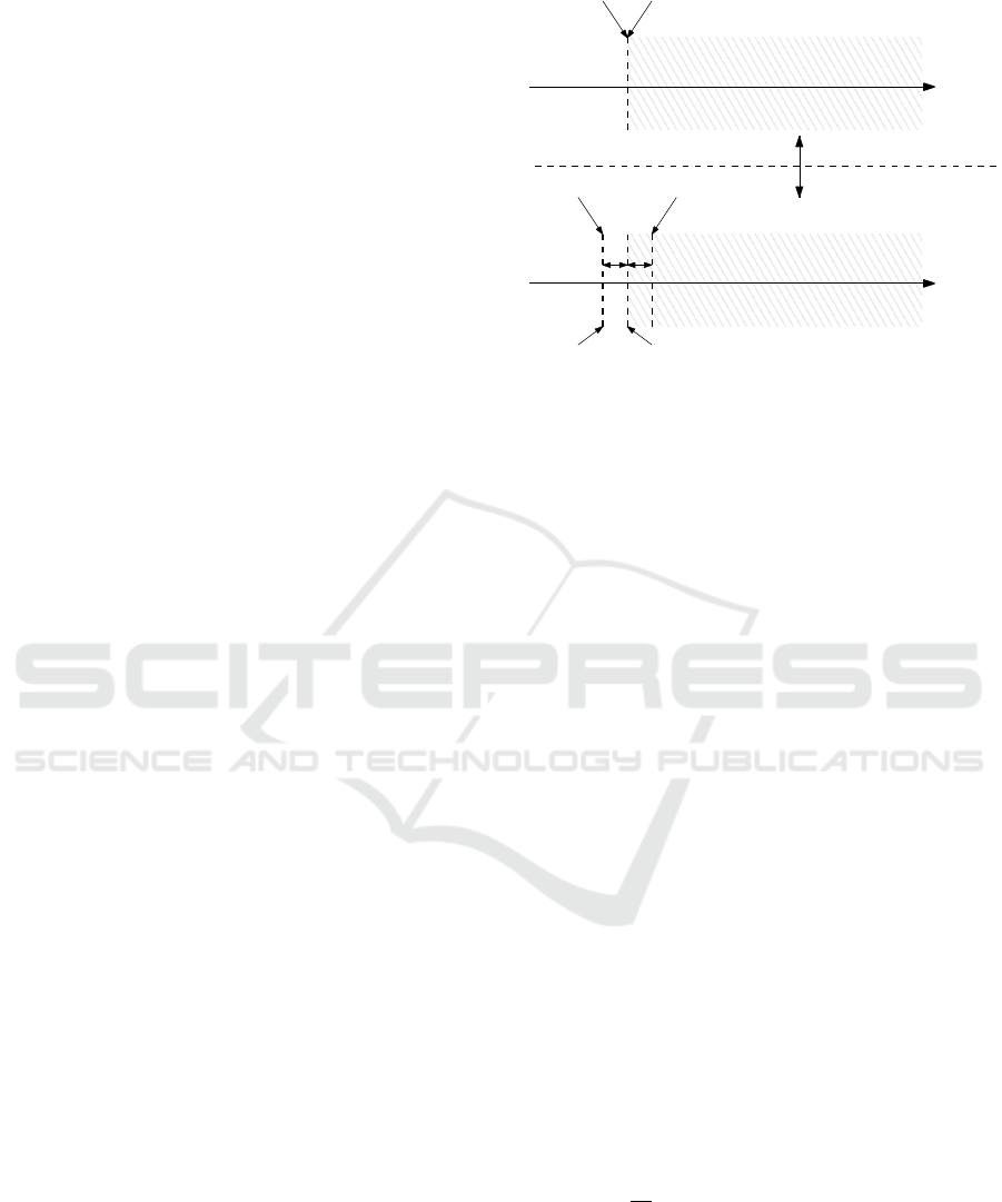
Update if

Update to

Update if

Update to

u,j

b,j



IC,j

− B



> 0

IC,j



IC,j

− B



> 0

IC,j

Without Update Heuristic

With Update Heuristic

Figure 1: Schematic illustration of the update heuristic.

3.3 Upper-Bounding the Computational

Load

Since the algorithm is utilized for model learning,

we can expect that our measurements, in majority,

do not violate our constraints, but the constraint in-

tegration rather improves the speed at which learning

takes place. To further reduce the maximum computa-

tional load per time step, we upper-bound the sequen-

tial pseudo-measurement updates per time step to

˜n

≤ n

. Practice has shown that in cases where the

actual hidden function is close to the bounds, noise

and numerical errors may lead to repetitive updates

w.r.t. certain constraints. In combination with the

upper-bounding of the pseudo-measurement updates

per time step, this may lead to cases where certain

constraints are not considered altogether. Thus, we in-

troduce an additional heuristic to enable a hysteresis-

like behavior: As illustrated in Fig. 1, we only update

if s

( j) − B

) > δ

b, j

. Moreover, we update to the

value

= B

−δ

u, j

, where δ

b, j

≥ 0 and δ

u, j

≥ 0 are

both small non-negative constants.

3.4 GP Monotonicity Assumptions as

Constraints

Monotonicity assumptions on a real, continuously

differentiable function z

(ζ

ζ) can be stated as inequal-

ity constraints of its partial derivatives w.r.t. its in-

puts, e.g.

∂z

∂ζ

≷ 0. According to the derivation in

(McHutchon, 2015), the mean values of the partial

derivative of a GP with SE kernels in the test grid X

Recursive Gaussian Process Regression with Integrated Monotonicity Assumptions for Control Applications

343

w.r.t. the input ζ

i,k

is given by

∂µ

∂ζ

i,k



−



i,k

− X



⊙ k(X

, X



· K



{z }

IC,l,k

·µ

(12)

where ⊙ denotes the Schur- or Hadamard product.

This function is linear in the mean values of the

RGP. For a constant test grid

X, the linear gain ma-

trix H

IC,l,k

is also time-invariant. For simplicity, we

only consider one monotonicity assumption per di-

mension, where l = 1, . . . , n

with n

≤ n

indicate

the input dimensions for which monotonicity assump-

tions exist. Consequently, each dimension is charac-

terized by only one set of values s

, B

, δ

B,l

and δ

U,l

As a constant test grid is considered for the mono-

tonicity, we can state the mean values of the partial

derivatives at the test vector grid using linear pseudo-

measurement matrices. They can be calculated by

means of

∂µ

∂ζ



−



− X



⊙ k(

X, X



· K



| {z }

IC,l

·µ

(13)

for all dimensions l that comply with monotonicity

assumptions. Here, the matrices H

IC,l

can be calcu-

lated ofﬂine.

As conﬁrmed in a comparison with the exact co-

variance of the partial derivative, see (McHutchon,

2015), the usage of these measurement functions

for the covariance prediction of the partial derivative

leads to further linearization errors. This error van-

ishes if

X = X

X holds. In the following, we therefore

choose the monotonicity test vector grid equal to the

basis vector grid – which is reasonable for most ap-

plications anyway.

3.5 Inequality Constraints on the GP

Output

Even though it is not employed in this paper, the

consideration of inequality constraints on GP out-

puts is included here for completeness. Like the

monotonicity constraints, output constraints are eval-

uated on a grid. If the chosen test grid is also

identical to the basis vector grid, the corresponding

output equation becomes µ

k+1

= J

X)µ

k+1

. Since

X) = k(X

X, X

X)K

= I

I holds, the respective pseudo-

measurement matrix becomes the identity matrix

= I

I and leads to the simpliﬁcation t

= µ

k+1

Please note that for soft GP output constraints, other

measures, like a bounding of the measurements y

the RGP mean values µ

, might be more efﬁcient and

effective.

3.6 Summary of GP Monotonicity

Constraints

This section summarizes the pseudo-measurement

updates for constraints related to monotonicity as-

sumptions in the RGP. The extended RGP algorithm

will in the following referred to as RGPm. Please

note that the index k denoting the time step is omitted

for simplicity. In addition to the ofﬂine precomputa-

tions (2) for the standard RGP in Sec. 2, the following

measurement matrices need to be calculated for each

input dimension with a monotonicity assumption:

For l = 1, . . . , n

IC,l



−



− X



⊙ K



· K



. (14)

Also the boundaries

= B

− δ

u,l

and δ

b,l

for

the update heuristic as well as the upper limits per

dimension ˜n

IC,l

have to be deﬁned.

For each time step k, after the evaluation of the

RGP inference (3) and update steps (4) from Sec. 2,

the pseudo-measurement update is computed as

follows:

Set C

1,1

= C

k+1

and µ

1,1

= µ

k+1

For l = 1, . . . , n

Evaluate t

= H

IC,l

l,1

, with H

IC,l

IC,l,1

, h

IC,l,2

, ..]

and set counter m = 1.

For j = 1, . . . , n

IC,l

If s

( j) −

) > δ

b,l

and m ≤ ˜n

IC,l

: , (15)

l, j

= C

l, j

IC,l, j

l, j

IC,l, j

+ r

)

−1

l, j+1

= µ

l, j

−

l, j

IC,l, j

l,1

−

)

l, j+1

= C

l, j

−

l, j

IC,l, j

l, j

m = m + 1

l+1,1

= µ

l, ˜n

IC,l

and C

l+1,1

= C

l, ˜n

IC,l

Set µ

k+1

= µ

, ˜n

IC,l

, but reset C

k+1

= C

1,1

3.7 Discussion

In general, a consideration of monotonicity con-

straints with a test vector grid unequal to the basis

vector grid is possible and was successfully imple-

mented. It tends to be, however, numerically unsta-

ble, most likely due to linearization errors w.r.t. the

covariance prediction.

As pointed out, the implemented monotonicity

constraints are only soft constraints. This means in

practice that the GP will adhere to the measurements

if these consistently contradict the monotonicity as-

sumptions. This scenario would be caused by wrong

ICINCO 2025 - 22nd International Conference on Informatics in Control, Automation and Robotics

344

assumptions regarding either the monotonicity itself

or the measurement quality. Although still not guar-

anteeing constraint satisfaction, a safety margin can

be added by changing B

accordingly. For safety-

critical constraints, an additional evaluation on a ﬁner

grid as well as a subsequent output correction may be

useful.

A UKF may be more suited for handling the non-

linearities in the presented pseudo-measurement up-

date. Nevertheless, it would prevent most of the re-

formulations which facilitate the envisaged real-time

implementation. Consequently, it was not considered

further.

Please note that piece-wise monotonicity can also

be addressed as long as the regions are deﬁnable

through sets of basis vector points. This variation

and the direct output constraints in Subsec. 3.5 have

already been successfully validated but are not de-

scribed for the sake of brevity.

Please note that the sequential update of the EKF

involves an additional condition for the equivalence to

a batchwise update. Here, the linearization point has

to be identical. This condition is fulﬁlled within each

input dimension by introducing the intermediary vari-

ables t

and t

in Subsecs. 3.2 and 3.4, respectively. It

is, however, not fulﬁlled over all input dimensions l in

Subsec. 3.4. Thus, even without the bounded number

of updates and the update heuristic, a slight deviation

is present between the sequential EKF and the batch-

wise EKF if several monotonicity assumptions apply.

4 VALIDATION BASED ON

SIMULATIONS

As a ﬁrst validation example, the hidden static func-

tion z

= 2(1 + 0.1ζ

+ ζ

) is learned. The input ζ

is picked from a random uniform distribution over the

complete input range ζ

∈ [−1, 1]. Zero-mean Gaus-

sian white noise with a variance of σ

= 1e − 2 is

added to the measured output y

The RGP hyperparameters remain constant and

are chosen as follows: L = 3, σ

= 1e1, and N = 21.

Obviously, the hidden function is strictly monoton-

ically increasing, so

∂z

∂ζ

> 0, B

= 0, and s

= −1

hold. The pseudo-measurement noise is chosen as

= 1e − 8.

4.1 Simulation Results

In Fig. 2, the hidden function z and its learned recon-

structions z

RGPm

and z

RGP

– with and without mono-

tonicity assumptions – are depicted after ﬁve noisy

-1 -0.8 -0.6 -0.4 -0.2 0 0.2 0.4 0.6 0.8 1

-1

Figure 2: RGP and RGPm outputs in comparison with the

hidden function z after 5 time steps.

measurements y

. It becomes obvious that the RGPm

algorithm works properly. In this example, it is ca-

pable of enforcing strict monotonicity over the whole

input range, while the curve is not signiﬁcantly al-

tered in the vicinity of the actual measurement points.

The result represents a clearly better ﬁt in comparison

with the classical RGP – especially in regions where

still no measurements are available.

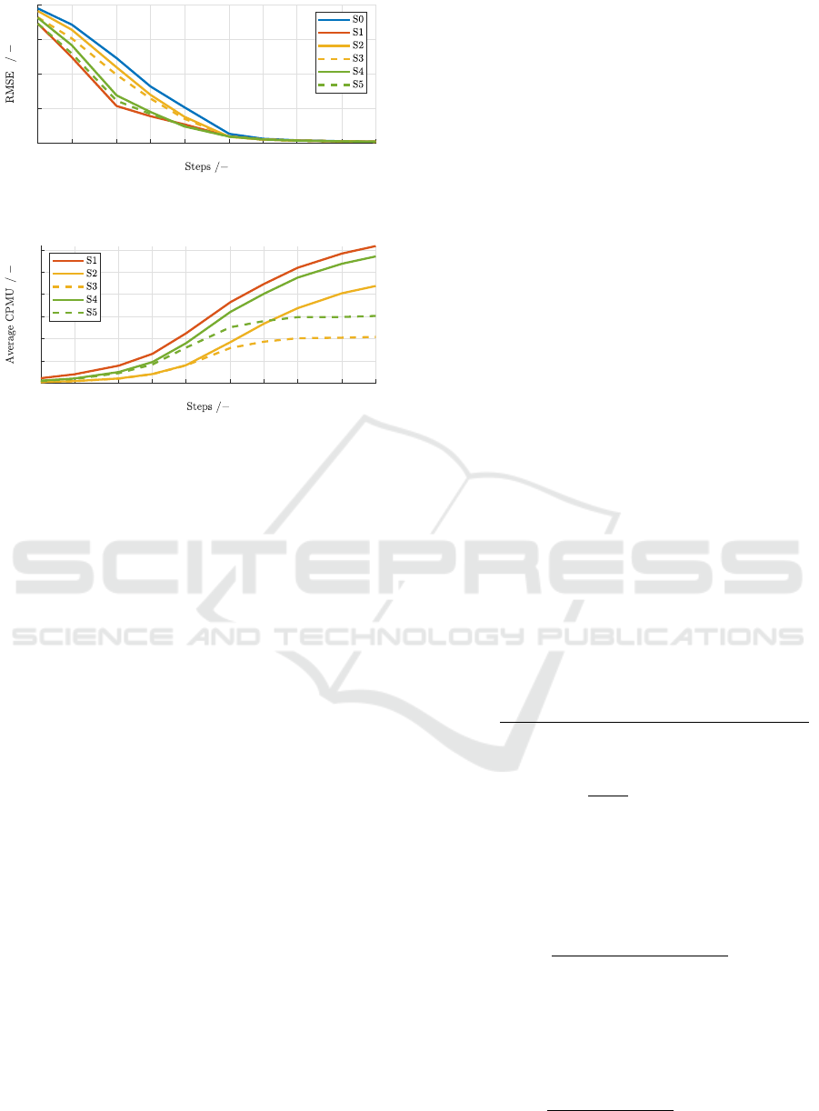
For a statistical validation of the algorithm and an

assessment of the impact of the adaptations, we inves-

tigate six different variants of the algorithm:

S0 Pure RGP

S1 unlimited ˜n

= n

RGPm with δ

= 0 and δ

= 0

S2 ˜n

= 2 limited RGPm with δ

= 0 and δ

= 0

S3 ˜n

= 2 limited RGPm with boundary heuristic

= 1e − 1 and δ

= 1e − 1

S4 ˜n

= 5 limited RGPm with δ

= 0 and δ

= 0

S5 ˜n

= 5 limited RGPm with boundary heuristic

= 1e − 1 and δ

= 1e − 1

For each scenario, 500 simulation runs are con-

ducted with the described uniform random input and

the noisy output. After k = 1, 2, 5, . . . , 1000 steps, the

root mean-squares error (RMSE) between the learned

function of each variation, compared to the hidden

function over the complete input range, is calculated.

This RMSE is again averaged over all 500 simula-

tions and depicted in Fig. 3. Fig. 4 shows the aver-

age cumulative number of pseudo-measurement up-

dates (CPMU) that were conducted for the alterna-

tives S1,...,S5.

All RGPm variants perform better than the classi-

cal RGP. This advantage vanishes after a certain num-

ber of steps, and all the RMSE converge to the same

value. This could be expected because the monotonic-

ity assumptions are valid and should be represented

on average in the measurements.

It can be seen that a tighter limit on the number of

pseudo-measurement updates per time step is gener-

ally a trade-off w.r.t. the performance. Accordingly,

S1 is better than S4 and S2. In the current applica-

tion, the improvement from S4 to S1 is however quite

Recursive Gaussian Process Regression with Integrated Monotonicity Assumptions for Control Applications

345

1 2 5 10 20 50 100 200 500 1000

0.5

1.5

Figure 3: Average RMSE for 500 simulation runs of the

different RGP and RGPm variants.

1 2 5 10 20 50 100 200 500 1000

100

150

200

250

300

Figure 4: Average cumulative pseudo-measurement updates

(CPMU) for 500 simulation runs of the different RGPm

variants.

small, and reverses slightly around 20 steps. This last

effect may stem from numerical errors that could be

related to the higher number of pseudo-measurement

updates.

The heuristic approach of including outer/inner

boundaries resulted in signiﬁcant improvements in the

RMSE. The reduced repeated pseudo-measurement

updates w.r.t. certain constraints are clearly visible in

Fig. 4. While S1, S2 and S4 still perform pseudo-

measurement updates after 1000 steps, the update

heuristic leads to a converging CPMU for S3 and S5,

which means that no more pseudo-measurement up-

dates are performed after a certain point. Whereas the

real-time capability is only inﬂuenced by the maxi-

mum number of updates per time step, the reduced

computational load can be seen as an additional ben-

eﬁt.

5 EXPERIMENTAL RESULTS

FOR A VAPOR COMPRESSION

CYCLE

In this chapter, the functionality of the proposed

method is investigated in a real-time application – a

counterﬂow evaporator as a subsystem of a VCC. As

discussed in detail in (Husmann et al., 2024a) and

(Husmann et al., 2024b), heat transfer values, espe-

cially in the presence of phase changes, depend on

process parameters and are hard to determine. In

(Husmann et al., 2024b), integral feedback was ap-

plied directly affecting the heat transfer value and

combined with a partial IOL. In addition to a stability

proof also the convergence of integrator state towards

the actual heat transfer value was proven. In this paper

we want to leverage the integrator steady state to learn

a RGP model for the heat transfer value that depends

on several process parameters. The aim is to use the

RGP model in parallel to the integrator feedback to

further improve the transient control behavior.

The algorithm was implemented on a test rig at

the Chair of Mechatronics at the University of Ro-

stock. The utilized hardware, a Bachmann PLC

(CPU:MH230), runs at a sampling time of 10ms. The

test rig is fully equipped with sensors, an electronic

expansion valve as well as a compressor with a vari-

able frequency drive. Please refer to (Husmann et al.,

2024a) and (Husmann et al., 2024b) for further details

about the test rig.

5.1 Partial IOL Control

As the partial IOL is described in detail in (Husmann

et al., 2024b), we only want to give a brief overview

in this paper. The envisioned control structure is de-

picted in Fig. 5. As shown, the control inputs are

given by the expansion valve opening u

and the com-

pressor speed u

. The control outputs are chosen as

the evaporator mean temperature y

= T

Evap

and the

superheating enthalpy y

= ∆h

after the evaporator.

The control-oriented evaporator model, ﬁrst derived

in (Husmann et al., 2023), is governed by the follow-

ing two ODEs

Evap

˙m

Evap,in

− ˙m

Evap,out

Evap

−( ˙m

− ˙m

Evap

(16)

and

Evap

( ˙m

− ˙m

) . (17)

Here, the ﬁrst state equation is affected by an uncer-

tain convective heat ﬂow

Evap

= α · α

norm

· A

Evap

· (T

− T

Evap

) (18)

with α

norm

as a normalization factor. The input-

dependent mass ﬂows are given by

˙m

= ζ

Cond,out

Cond

− p

Evap

) · u

(19)

and

˙m

= ˆm

Rev

. (20)

Both outputs can be expressed in terms of the state

variables. The second output is given by

lin,2

= ∆h

Evap

−(1−w

Evap,in

− h

Evap,sat

Evap

(21)

ICINCO 2025 - 22nd International Conference on Informatics in Control, Automation and Robotics

346

IOL

Physical

System

∆h

−

∆h

sh,d

Filter

m,f

ˆα

RGPm

ˆα

RGP/

RGPm

Figure 5: Nonlinear tracking control structure.

and its ﬁrst time derivative becomes

˙y

lin,2

Evap

−

1−w

Evap,in

−

∂h

sat

∂T



Evap

(22)

which lead to a relative degree of one. Whereas the

inverse dynamics is determined for both control in-

puts in the standard IOL proposed in (Husmann et al.,

2023), the partial IOL used here leverages the inverse

dynamics of the control input u

= b

(.)

−1

[υ

− a

(.) − b

(.)u

] , (23)

and considers the second input u

as a measurable

disturbance. Please note that a secondary controller

needs to be implemented for the ﬁrst control output

= T

Evap

, see (Husmann et al., 2024b). In this pa-

per, however, the control input u

is assumed as given

because it has no relevance for the presented algo-

rithm. The partial IOL is completed with a stabilizing

feedback υ

= k

, with e

= y

2,d

− y

. Here the

nonlinear feedback from (Husmann et al., 2024b) is

utilized. The introduction of a parameter update law

for the heat transfer value

α = −k

2,d

− y

), which

corresponds to integral control action w.r.t.

α, dra-

matically increases the performance and guarantees

steady-state accuracy as shown in (Husmann et al.,

2024b). Since the integrator state

α was proven to

converge to an exact representation of the lumped heat

transfer value in the control-oriented model, it is suit-

able for the training of a model.

5.2 RGPm Implementation

As input variables for the GP model, the compres-

sor speed u

and the superheating enthalpy y

= ∆h

are chosen, i.e.,

= z(u

, ∆h

). As known from

our own experiments and from the literature, the in-

equalities

∂α

∂u

> 0 and

∂α

∂∆h

< 0 hold. Consequently,

they are included as monotonicity assumptions in the

RGPm algorithm. The evaluation of the GP model is

conducted with the reference value y

d,2

instead of the

current one, i.e.,

= z(u

, ∆h

SH,d

). Thereby, any

additional feedback is avoided, and the GP model ob-

tains a pure feedforward structure w.r.t. its evaluation.

This prevents stability issues.

The RGP and RGPm algorithms are implemented

with basis vector dimensions of N

= 5 and N

= 5

for the respective GP inputs, which results in N

25 basis vector points. The monotonicity update is

bounded to n

= n

= 5 steps per dimension and per

time step. The parameters for the update heuristics are

deﬁned as follows: δ

u,1

= δ

u,2

= 0 and δ

b,1

= δ

b,2

2e − 6. The pseudo-measurement noise is chosen as

= r

= 1e −8, and the length scale is set to L = 1.5.

The signing variables for the respective monotonicity

assumptions are given by s

= −1 and s

= 1 and the

safety margins are disabled, so B

= B

= 0.

To ensure that the integrator state is only utilized

in the vicinity of it’s equilibrium state, we employ

a heuristic which only enables the RGP update if

| < 1 holds for 10 consecutive seconds. The numer-

ical values in this heuristic mark a trade-off between

learning speed and accuracy. With a larger error mar-

gin or a shorter time horizon, more data qualiﬁes for

training. However, the considered data might also re-

late to system states further away from the equilib-

rium.

5.3 Results

To illustrate the functionality and advantages of the

RGPm algorithm, two consecutive experiments with

the same step-wise u

-trajectory are performed: the

ﬁrst one for y

2,d

= 14, the other one for y

2,d

= 7. The

RGPm algorithm is trained online during both exper-

iments – without applying its output value to the con-

troller. For a comparison, the RGP algorithm is later

trained ofﬂine on the same data. The results after the

ﬁrst and second experiment are depicted for both al-

gorithms in Fig. 6. Since the monotonicity updates

for the covariance matrix are discarded at the end

of each time step, both algorithms lead to the same

covariance, so that only one is depicted per experi-

ment. In the upper right picture of Fig. 6, the training

region during the experiment becomes obvious, be-

cause the covariance is small there. When comparing

the mean values for the RGPm (upper left) and RGP

(upper middle), it becomes evident that the learned

model within the input region used for the training is

nearly identical. Outside of this region, however, the

shapes vary drastically. While the monotonicity as-

sumptions in the RGPm model lead to a physically

viable model shape, this cannot be stated for the stan-

dard RGP model. Here, the overall shape is only de-

ﬁned by the limited amount of data available in the

non-trained region. As shown in the comparison of

the trained models after the second experiment for

both RGPm (lower left) and RGP (lower middle), the

differences between the models decline with the avail-

ability of data. This reinforces the ﬁndings from the

simulation study.

Recursive Gaussian Process Regression with Integrated Monotonicity Assumptions for Control Applications

347

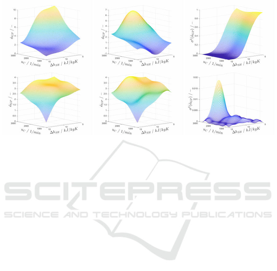
Figure 6: GP model predictions from left to right: RGPm (online), RGP (ofﬂine comparison for same data) and covariances

of both variants. From top to bottom: after the ﬁrst u

-trajectory for y

2,d

= 14, and after the second u

-trajectory for y

2,d

= 7.

The softness of the constraints in the RGPm algo-

rithm becomes clear for low superheating and large

compressor speeds. Here, the monotonicity con-

straints are slightly violated, however much less than

in the standard RGP algorithm. The violation may be

ﬁxed by safety margins and a more involved heuristic

for the RGP update.

The evaluation of the overall control performance

with the trained model is outside of the scope of

this paper, since a more detailed comparison would

need additional concepts and algorithms, e.g. suitable

training strategies. A quick validation of the RGPm

model after the second experiment, depicted in Fig.

6 (lower left corner), can be performed by deactivat-

ing the integrator feedback control and running a u

test trajectory together with a learned

and with a

constant α. Here, for a reference value of y

= 13,

which wasn’t used for the training, a 28 % reduc-

tion in RMSE could be achieved, which represents a

promising ﬁrst result for the application of the trained

RGPm model.

6 CONCLUSIONS AND

OUTLOOK

This paper presents an extension of the recursive

Gaussian Process regression (RGP) algorithm to en-

force (soft) constraints during an online training.

Here, the consideration of monotonicity assumptions

in the GP model is emphasized as well as their imple-

mentation as constraints. The algorithm is statistically

validated in simulations. Moreover, different sim-

pliﬁcations are introduced to enable a real-time use,

and their effect on the performance is investigated.

A real-time implementation on a test rig is presented

afterwards, where the learning of heat transfer value

models for an evaporator is considered. The evap-

orator is a main component of a vapor compression

cycle operated by a previously published partial IOL.

Here, the extension of a standard RGP regression by

monotonicity constraints results in a signiﬁcantly bet-

ter modeling – especially if few data is available.

A combination of the extension presented in this

paper with the Kalman Filter integration of the RGP

(KF-dRGP), is straightforward and allows for an RGP

training with constraints if the output of the hid-

den function is not directly measurable. For systems

where a hard constraint satisfaction is crucial, further

investigations are still necessary. As discussed ear-

lier, an additional safety step with a calculation of the

constraint satisfaction on a ﬁner grid could be suit-

able. As mentioned in Sec. 5, the full integration of

the GP model within the partial IOL for the VCC con-

trol necessitates further work. It is obviously desir-

able, for example, to simultaneously learn and apply

the learned model. This does, however, introduce an

additional feedback loop into the system, which may

affect the stability. Here, the presented output and

monotonicity bounds mark important tools. Given

promising ﬁrst results, steps in this direction will be

topics of future work.

ICINCO 2025 - 22nd International Conference on Informatics in Control, Automation and Robotics

348

REFERENCES

Beckers, T., Seidman, J., Perdikaris, P., and Pappas, G. J.

(2022). Gaussian process port-hamiltonian systems:

Bayesian learning with physics prior. In 2022 IEEE

61st Conference on Decision and Control (CDC),

pages 1447–1453.

Blum, M. (1957). Fixed memory least squares ﬁlters using

recursion methods. IRE Transactions on Information

Theory, 3(3):178–182.

Desai, S. A., Mattheakis, M., Sondak, D., Protopapas, P.,

and Roberts, S. J. (2021). Port-hamiltonian neural net-

works for learning explicit time-dependent dynamical

systems. Physics Review E, 104:034312.

Gupta, N. and Hauser, R. (2007). Kalman ﬁltering with

equality and inequality state constraints.

Haseltine, E. L. and Rawlings, J. B. (2005). Critical evalua-

tion of extended Kalman ﬁltering and moving-horizon

estimation. Industrial & Engineering Chemistry Re-

search, 44(8):2451–2460.

Huber, M. F. (2013). Recursive Gaussian process re-

gression. In 2013 IEEE International Conference

on Acoustics, Speech and Signal Processing, pages

3362–3366.

Huber, M. F. (2014). Recursive Gaussian process: On-line

regression and learning. Pattern Recognition Letters,

45:85–91.

Husmann, R., Weishaupt, S., and Aschemann, H. (2023).

Nonlinear control of a vapor compression cycle by

input-output linearisation. In 27th International Con-

ference on Methods and Models in Automation and

Robotics (MMAR), pages 193–198.

Husmann, R., Weishaupt, S., and Aschemann, H. (2024a).

Control of a vapor compression cycle based on a

moving-boundary model. In 2024 28th International

Conference on System Theory, Control and Comput-

ing (ICSTCC), pages 438–444.

Husmann, R., Weishaupt, S., and Aschemann, H. (2024b).

Nonlinear control of a vapor compression cycle based

on a partial IOL. In IECON 2024 - 50th Annual

Conference of the IEEE Industrial Electronics Soci-

ety, pages 1–6.

Husmann, R., Weishaupt, S., and Aschemann, H. (2025).

Direct integration of recursive Gaussian process re-

gression into extended Kalman ﬁlters with applica-

tion to vapor compression cycle control. In 13th IFAC

Symposium on Nonlinear Control Systems NOLCOS

2025.

Jain, L. C., Seera, M., Lim, C. P., and Balasubramaniam,

P. (2014). A review of online learning in supervised

neural networks. Neural computing and applications,

25:491–509.

Julier, S. J. and Uhlmann, J. K. (1997). A new ex-

tension of the Kalman ﬁlter to nonlinear systems.

In Proc. of AeroSense: The 11th Int. Symp. on

Aerospace/Defence Sensing Simulation and Controls.

Kalman, R. E. (1960). A new approach to linear ﬁltering

and prediction problems. Transactions of the ASME–

Journal of Basic Engineering, 82(Series D):35–45.

McHutchon, A. J. (2015). Nonlinear modelling and con-

trol using Gaussian processes, chapter A2, pages 185–

192.

Nocedal, J. and Wright, S. J. (2006). Numerical Opti-

mization, chapter 16.5, pages 467–480. Springer New

York, NY.

Qui

nonero-Candela, J. and Rasmussen, C. E. (2005). A uni-

fying view of sparse approximate Gaussian process

regression. Journal of Machine Learning Research,

6:1939–1959.

Sch

urch, M., Azzimonti, D., Benavoli, A., and Zaffalon,

M. (2020). Recursive estimation for sparse Gaussian

process regression. Automatica, 120.

Simon, D. (2006a). Optimal State Estimation, chapter 7.5,

pages 212–222. John Wiley & Sons, Ltd.

Simon, D. (2006b). Optimal State Estimation, chapter 6.1,

pages 150–155. John Wiley & Sons, Ltd.

Tully, S., Kantor, G., and Choset, H. (2011). Inequality

constrained Kalman ﬁltering for the localization and

registration of a surgical robot. In 2011 IEEE/RSJ In-

ternational Conference on Intelligent Robots and Sys-

tems, pages 5147–5152.

Veiga, S. D. and Marrel, A. (2020). Gaussian process re-

gression with linear inequality constraints. Reliability

Engineering & System Safety, 195:106732.

Recursive Gaussian Process Regression with Integrated Monotonicity Assumptions for Control Applications

349