Uncertainty Estimation and Calibration of a Few-Shot Transfer

Learning Model for Lettuce Phenotyping

Rusith Chamara Hathurusinghe Dewage

1,2 a

, Habib Ullah

1 b

, Muhammad Salman Siddiqui

1 c

Rakibul Islam

2 d

and Fadi-Al Machot

1 e

Faculty of Science and Technology, Norwegian University of Life Sciences, P.O. Box 5003, NO-1432 ,

As, Norway

Photosynthetic AS, Sjøskogenveien 5, 1407 Vinterbro, Norway

Keywords:

Few-Shot Learning, Transfer Learning, Uncertainty Estimation, Calibration.

Abstract:

Computer vision-assisted automatic plant phenotyping in controlled environment agriculture (CEA) remains a

signiﬁcant challenge due to the scarcity of labeled data from growing conditions. In this work, we investigate

few-shot transfer learning for estimating the maximum width of lettuce from cropped and segmented images

exhibiting non-uniform spatial distribution. The dataset presents additional complexity as images are cap-

tured using a wide-angle, off-center camera. We systematically investigate backbone architectures (ResNet,

EfﬁcientNet, MobileNet, DenseNet, and Vision Transformer) and perform various data augmentation strate-

gies and regression head designs to identify optimal conﬁgurations under few-shot conditions. To enhance

predictive reliability, we employ post-hoc uncertainty estimation using Monte Carlo (MC) dropout and con-

formal prediction, and further evaluate model calibration to analyze alignment between predicted uncertainties

and empirical errors. Our best model, based on Vision Transformer Huge with 14×14 patch size (ViT-H/14),

achieved a root mean square error (RMSE) of 14.34 mm on the test set. For uncertainty estimation, MC

dropout achieved a miscalibration area of 0.19, an average prediction interval width of 27.89 mm, and an

empirical coverage of 73% at the nominal 90% conﬁdence level. Our results highlight the importance of back-

bone selection, augmentation, and head architecture on model generalization and reliability. This study offers

practical guidelines for developing robust, uncertainty-aware few-shot models for plant phenotyping, enabling

more trustworthy deployment in CEA applications.

1 INTRODUCTION

Deep learning is widely used in many domains, fa-

cilitating automated analysis of complex visual data.

In controlled environment agriculture (CEA), deep

learning models have shown promise in tasks such

as crop monitoring, yield estimation, and precision

agriculture (Wang et al., 2022b; Mokhtar et al., 2022;

Zhang and Li, 2022). Nevertheless, the success of

these applications often depends on good quality,

large, and labeled datasets. Collecting useful data and

labeling it appropriately requires time and human re-

sources. Few-shot learning offers an alternative train-

https://orcid.org/0009-0004-6144-7807

https://orcid.org/0000-0002-2434-0849

https://orcid.org/0000-0002-6003-5286

https://orcid.org/0000-0002-7174-9225

https://orcid.org/0000-0002-1239-9261

ing approach by enabling models to learn from a lim-

ited number of samples. Despite their strong predic-

tive powers, deep learning models need an assessment

of their uncertainty to ensure reliability in real-world

applications. Without appropriate uncertainty estima-

tion, decisions based on predictive models may be un-

reliable, particularly in areas such as CEA, where un-

reliable predictions can result in huge ﬁnancial losses.

In the cases of insufﬁcient labeled data, few-shot

learning enables training a model with minimal sam-

ples by utilizing pre-trained deep-learning architec-

tures. The key objectives of this research are to ap-

ply few-shot transfer learning to predict the maximum

width of lettuce from a limited number of segmented

images, quantify uncertainty in the model’s predic-

tions on the test dataset, and evaluate model calibra-

tion. To achieve these objectives, we utilized a dataset

of lettuce images captured at various growth stages in

a controlled environment. The dataset also included

388

Dewage, R. C. H., Ullah, H., Siddiqui, M. S., Islam, R. and Machot, F.-A.

Uncertainty Estimation and Calibration of a Few-Shot Transfer Learning Model for Lettuce Phenotyping.

DOI: 10.5220/0013743600004000

Paper published under CC license (CC BY-NC-ND 4.0)

In Proceedings of the 17th International Joint Conference on Knowledge Discovery, Knowledge Engineering and Knowledge Management (IC3K 2025) - Volume 1: KDIR, pages 388-397

ground-truth measurements of the maximum lettuce

width.

This study enhances the domain of deep learning

uncertainty estimation in agricultural applications by

ensuring that deep learning models generate predic-

tions that are both accurate and reliable.

2 RELATED WORK

The success of deep learning is mainly driven by the

availability of extensive datasets, enhanced process-

ing capabilities, and improvements in training tech-

niques. Nonetheless, deep learning models frequently

encounter difﬁculties when faced with limited train-

ing data, and they cannot fundamentally quantify un-

certainty in their predictions, hence constraining their

use in essential ﬁelds such as healthcare and agricul-

ture.

Few-shot learning (FSL) has emerged as a pow-

erful approach in agriculture to address the challenge

of limited labeled data. Ruan et al. applied meta-

learning with hyperspectral imaging to detect drought

and freeze stress in tomatoes using as few as eight tar-

get domain samples, achieving superior performance

over traditional methods (Ruan et al., 2023). Lager-

gren et al. used FSL with convolutional neural net-

works (CNNs) to segment leaf morphology and vena-

tion traits from high-resolution ﬁeld images, enabling

efﬁcient phenotyping and genetic analysis with min-

imal annotation (Lagergren et al., 2023). FSL has

also shown promise in classiﬁcation tasks and im-

proving model robustness. Belissent et al. combined

transfer and zero-shot learning for weed classiﬁca-

tion, showing ResNet50’s effectiveness on the Toma-

toWeeds dataset and potential for identifying unseen

species (Belissent et al., 2024). Wang et al. reviewed

FSL techniques such as Siamese networks, prototyp-

ical networks, and GANs for plant disease and pest

recognition, presenting their high accuracy with lim-

ited data (Wang et al., 2022a). Luo et al. high-

lighted the importance of uncertainty estimation and

model calibration in CEA, suggesting FSL combined

with post-training techniques can enhance real-world

decision-making (Luo et al., 2023).

A signiﬁcant advancement of FSL is few-shot

transfer learning (FSTL), which has demonstrated

considerable performance in plant phenotyping and

other ﬁelds. Research has shown that ﬁne-tuning

CNNs using limited plant datasets can substantially

enhance accuracy and efﬁciency relative to training

from the ground up (Ojo and Zahid, 2022; Yang

et al., 2022). The recent paper by Hossen et al. re-

views the use of transfer learning (TL) in agricul-

ture, addressing data scarcity in the ﬁeld. Recent ad-

vances in agricultural applications have demonstrated

the effectiveness of TL using various foundation mod-

els. Classical CNNs such as VGG16, ResNet50/101,

AlexNet, and InceptionV3 have been widely adopted

for tasks like plant species recognition, disease de-

tection, pest classiﬁcation, and seedling identiﬁca-

tion, often achieving high accuracy even with limited

or complex datasets. Lightweight models like Mo-

bileNetV2/V3, SqueezeNet, and EfﬁcientNetB4 of-

fer improved efﬁciency and are particularly suited for

real-time or resource-constrained applications. Hy-

brid methods, including combinations with SVMs,

GANs, bilinear CNNs, and XGBoost, further en-

hance performance. Emerging architectures such

as DenseNet121, EfﬁcientDet, YOLOv5, DenseY-

OLOv4, Swin Transformer, and Xception have shown

promise in specialized tasks like crop-weed detection,

plant growth prediction, and nutrient deﬁciency anal-

ysis. These studies consistently report high F1-scores

and accuracy, underscoring TL’s critical role in devel-

oping scalable and effective models for smart agricul-

ture (Hossen et al., 2025).

Although FSL has successfully enhanced model

generalization, uncertainty quantiﬁcation continues to

pose a signiﬁcant barrier, as deep learning models

generally do not offer conﬁdence intervals for their

predictions. Uncertainty in deep learning is mainly

of two types: aleatoric, arising from inherent data

noise and irreducible by more data, and epistemic,

stemming from limited model knowledge that can be

reduced with additional data. While classiﬁcation

models estimate uncertainty via predicted class prob-

abilities, regression models often lack inherent un-

certainty quantiﬁcation (H

ullermeier and Waegeman,

2021). Bayesian Neural Networks address epistemic

uncertainty by modeling weight distributions, but are

computationally challenging, leading to approximate

methods such as Monte Carlo dropout, which uses

dropout at inference to mimic posterior sampling, and

conformal prediction, which provides formal predic-

tion intervals (Kendall and Gal, 2017).

Recent work in few-shot learning has emphasized

improving uncertainty estimation and calibration to

enhance model reliability under limited data condi-

tions. Chang et al. proposed BMLPUC, which com-

bines calibrated uncertainty with adaptive training

for accurate Remaining Useful Life (RUL) prediction

(Chang and Lin, 2025). Similarly, Ding et al. in-

troduced BA-PML, a probabilistic few-shot learning

approach leveraging Bayesian Seq2Sep modeling and

episodic training for improved uncertainty in machin-

ery prognostics (Ding et al., 2023).

Other approaches integrate novel uncertainty-

Uncertainty Estimation and Calibration of a Few-Shot Transfer Learning Model for Lettuce Phenotyping

389

aware mechanisms into classiﬁcation and vision-

language models. He et al. developed CLUR, us-

ing contrastive learning and pseudo uncertainty scores

for effective uncertainty estimation in few-shot text

classiﬁcation (He et al., 2023). Morales et al. pro-

posed BayesAdapter, a Bayesian extension to CLIP

adapters that captures predictive distributions and en-

hances calibration in vision-language tasks (Morales-

Alvarez et al., 2024). Park et al. introduced meta-

XB, improving conformal prediction by reducing pre-

diction set size while ensuring strong calibration via

adaptive non-conformal scoring (Park et al., 2023).

Iwata et al. presented a meta-learning strategy for cal-

ibrating deep kernel Gaussian Processes, using task-

shared encoders and GMMs to achieve efﬁcient and

well-calibrated few-shot regression (Iwata and Kuma-

gai, 2023).

3 METHODOLOGY

3.1 Data Collection and Preprocessing

The hydroponics lab, shown in Figure 2, served as

the primary experimental setup for this study. The

facility contains two independent chambers (zones),

which allow the simultaneous execution of two dif-

ferent plant growth protocols. These chambers reg-

ulate key environmental parameters, including light

intensity, water temperature, air temperature, nutri-

ent concentration, pH levels, carbon dioxide (CO

)

concentration, and relative humidity. A sensor sys-

tem continuously monitors and adjusts these condi-

tions to maintain predeﬁned target values. Through-

out the plant growth cycle, the system systematically

collects all sensor measurements. It captures plant

images using a wide-angle camera in the top corner

of each chamber and stores them in Firebase Realtime

Database and Storage.

We collected images from an experiment con-

ducted in the hydroponics lab, where we maintained

a high carbon dioxide concentration in Zone 1 and a

low concentration in Zone 2 while keeping all other

variables nearly constant. This variation in CO

lev-

els led to different lettuce growth rates between the

two chambers. We manually measured the maximum

width of the lettuce on the 11

, 13

, 16

, and 19

days of growth. After retrieving images from these

days, we cropped and annotated individual plants that

were not occluded using the VGG Image Annota-

tor (Dutta and Zisserman, 2019). We then created

masked images by setting background pixel values to

zero.

The dataset included 72 masked images of lettuce

Table 1: Means and standard deviations computed from the

ImageNet dataset used to normalize the pixel values in each

channel.

Channel Mean Standard Deviation

R 0.485 0.229

G 0.456 0.224

B 0.406 0.225

as shown in Figure 3. The distribution of maximum

lettuce widths are shown in Figure 4.

The images were ﬁrst padded to achieve a square

shape, ensuring that the longer dimension, either

width or height, determined the ﬁnal size. Follow-

ing this, they were resized to 224 × 224 pixels. To

standardize pixel intensity values, the images were

rescaled by dividing each channel’s pixel values by

255. Subsequently, normalization was performed us-

ing the mean and standard deviation values computed

from the ImageNet dataset (Deng et al., 2009), as pre-

sented in Table 1, for each channel.

The dataset was divided into three bins based on

the maximum width of the lettuce samples. Subse-

quently, it was split into training, validation, and test

sets in a 60:20:20 ratio using stratiﬁed sampling based

on the bin assignments, resulting in 42, 15, and 15

samples, respectively. The training and validation sets

were then used to select the backbone network, tune

data augmentation strategies, and optimize the model

head architecture.

3.2 Model Architecture

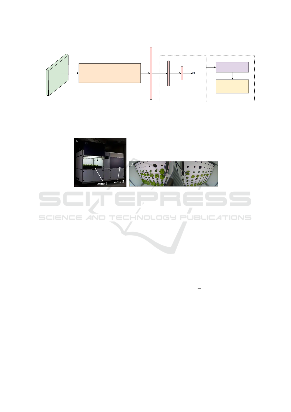
The overall model architecture is illustrated in Figure

1. Let x ∈ R

224×224×3

denote an input image and y ∈

R the corresponding maximum lettuce width.

We ﬁrst extract a feature vector z using a pre-

trained Vision Transformer (ViT-H/14) backbone

f (·; θ

z = f (x; θ

), z ∈ R

(1)

where θ

are the frozen backbone parameters and d is

the feature dimension.

The regression head comprises two fully-

connected layers with ReLU activation:

= ReLU (W

z + b

) (2)

ˆy = ReLU (W

+ b

) (3)

where W

∈ R

512×d

, b

∈ R

512

, W

∈ R

32×512

, b

∈

are trainable parameters.

Notation: ReLU(·) is the rectiﬁed linear unit acti-

vation function.

KDIR 2025 - 17th International Conference on Knowledge Discovery and Information Retrieval

390

Vision Transformer (ViT-H/14)

224

1280

512

Input: Normalized

Image (224x224x3)

Backbone Network

Embedding

Dense

Layer 1

Dense

Layer 2

Maximum

width

Regression Head

Monte Carlo Dropout

Conformal Prediction

Calibration Assessment

Prediction Interval

Calibration Curve

Uncertainty Estimation

Figure 1: Architecture of the proposed model. It takes a normalized segmented lettuce image as input and extracts features

using a Vision Transformer (ViT-Huge) with a 14×14 patch size. The extracted features are passed through two dense layers

with ReLU activation to predict the maximum lettuce width. Uncertainty estimation is performed using Monte Carlo dropout

and conformal prediction, resulting in prediction intervals. Model calibration is assessed via calibration curves.

Figure 2: Hydroponics lab exterior view (A). The lab has two independent chambers (zone 1 and zone 2) that enable simul-

taneous execution of different plant growth protocols. Hydroponics lab interior view (B). Plant images are captured using a

wide-angle off-center camera in each zone.

3.3 Training Procedure

We began by evaluating various pre-trained neural

network architectures to serve as feature extractors.

Speciﬁcally, we evaluated ResNet50, ResNet101,

EfﬁcientNetB0, MobileNetV2, DenseNet121, ViT-

B/16, and ViT-H/14. The Keras deep learning frame-

work (Chollet et al., 2015) was used to implement the

ﬁrst ﬁve models, while the ﬁnal two models were ac-

cessed via the PyTorch Image Models library (Wight-

man, 2019). These networks were used in a frozen

state (without updating their weights during training),

and the output features were fed into a minimal re-

gression head.

After selecting the backbone network, we inves-

tigated the effect of data augmentation on general-

ization performance. Several augmentation strategies

were evaluated, adding rotation, horizontal ﬂip, verti-

cal ﬂip, brightness, zoom in, zoom out, zoom in and

out, horizontal and vertical shift, and shear sequen-

tially starting from no augmentation. Each conﬁgura-

tion was evaluated while keeping the backbone frozen

and a minimal regression head. Five augmented ver-

sions were generated for each image. With the back-

bone and augmentation strategy ﬁxed, we explored

various conﬁgurations of the model head. Speciﬁ-

cally, we experimented with different numbers and

sizes of dense layers. Rectiﬁed Linear Unit (ReLU)

was used as the activation function.

Early stopping with a patience of 5 epochs was

employed during the hyperparameter tuning process

to avoid overﬁtting. The optimization was performed

using the ADAM optimizer (Kingma and Ba, 2014)

with a learning rate of 0.001 and a batch size of 8, due

to the small dataset size. The network was trained to

minimize mean squared error (MSE) over the training

set D = {(x

, y

)}

i=1

MSE

∑

i=1

( ˆy

− y

)

(4)

where ˆy

is given by Eq. 3. Performance was assessed

using the validation loss and R

score to identify the

most suitable hyperparameters.

The ﬁnal model architecture employed ViT-H/14

as the backbone, followed by two fully connected hid-

den layers comprising 512 and 32 neurons, respec-

tively. The data augmentation strategy included ran-

dom rotations within a range of ±40

◦

, random bright-

ness adjustments within ±0.1, and random horizontal

ﬂipping. The model’s performance was subsequently

Uncertainty Estimation and Calibration of a Few-Shot Transfer Learning Model for Lettuce Phenotyping

391

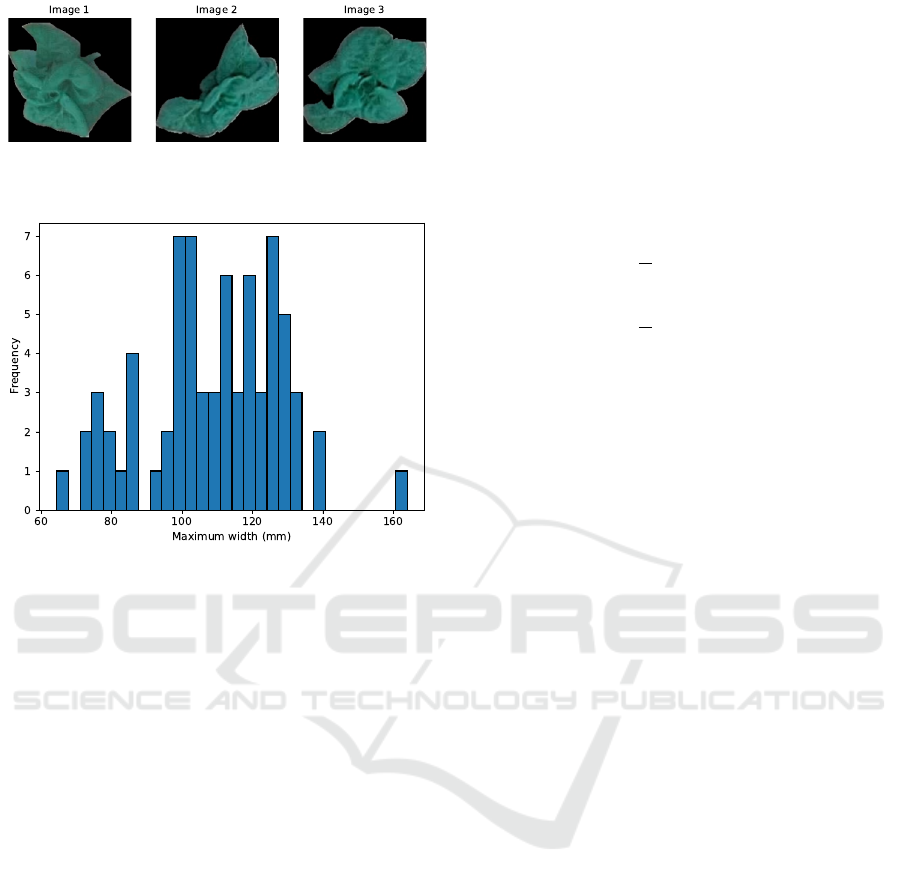
Figure 3: Few samples of masked lettuce images in the

dataset.

Figure 4: Distribution of maximum widths of lettuce in the

dataset.

evaluated on the test dataset.

3.4 Uncertainty Estimation

To quantify uncertainty using conformal prediction,

we employed the ”Naive” method, which calculates

nonconformity scores on a calibration set (Tibshirani,

2023).

Given a calibration set D

cal

, we compute absolute

residuals:

= |y

− ˆy

|, ∀(x

, y

) ∈ D

cal

(5)

For miscoverage rate α, let q

1−α

be the (1 − α)-

quantile of {r

}. The conformal prediction interval

for a new test sample x

new

is:

C(x

new

) = [ ˆy

new

− q

1−α

, ˆy

new

+ q

1−α

] (6)

where ˆy

new

is obtained by Eq. (3).

We computed the 95% prediction intervals using

a signiﬁcance level of 0.05 and using validation set

for computing nonconformity scores. Prediction in-

tervals were computed for the test data points and pre-

dictions and their 95% prediction intervals were plot-

ted.

To estimate uncertainty using MC dropout (Gal

and Ghahramani, 2016), we modiﬁed the model head

by incorporating a dropout layers with a dropout rate

of 0.1, positioned after the hidden layers. This modi-

ﬁed the model architecture Eq. 2 and Eq. 3 as follows,

where p denotes the dropout rate.

= Dropout (ReLU(W

z + b

), rate = p) (7)

ˆy = Dropout (ReLU (W

+ b

), rate = p) (8)

At inference, dropout remains enabled and the

model is sampled T times for each input, yielding pre-

dictions { ˆy

(t)

}

t=1

ˆy

∑

t=1

ˆy

(t)

(9)

ˆy

∑

t=1



ˆy

(t)

− µ

ˆy



(10)

where µ

ˆy

is the predictive mean and σ

ˆy

quantiﬁes

epistemic uncertainty. We plotted the predictions

and their 95% prediction intervals for the test dataset

assuming the predictions are normally distributed

around the mean.

Calibration diagrams were plotted for the predic-

tion intervals generated by both the MC dropout and

conformal prediction methods. The results were then

compared to evaluate their performance.

4 RESULTS

The ﬁnal model achieved an RMSE of 14.34 mm and

an R

value of 0.4464 on the test set. The average 90%

uncertainty intervals estimated by MC dropout and

conformal prediction were 27.89 mm and 27.74 mm,

respectively. Figure 5 shows the learning curve with

training and validation loss. The actual vs. predicted

maximum width of lettuce in the test set is shown in

Figure 6, where the ideal line represents perfect pre-

dictions. Figure 7 illustrates the test set predictions

along with 95% conﬁdence intervals estimated using

the MC dropout method. Figure 8 presents the 95%

uncertainty intervals estimated using the “Naive” con-

formal prediction method for the test set samples. Fi-

nally, Figure 9 displays the calibration plot for the un-

certainties estimated by MC dropout, while Figure 10

shows the calibration plot for the uncertainties esti-

mated by the “Naive” conformal prediction method.

5 DISCUSSION

To systematically explore the inﬂuence of various

architectural and training choices on model perfor-

mance, we employed a sequential hyperparameter

tuning approach. Given the limited size of our dataset,

KDIR 2025 - 17th International Conference on Knowledge Discovery and Information Retrieval

392

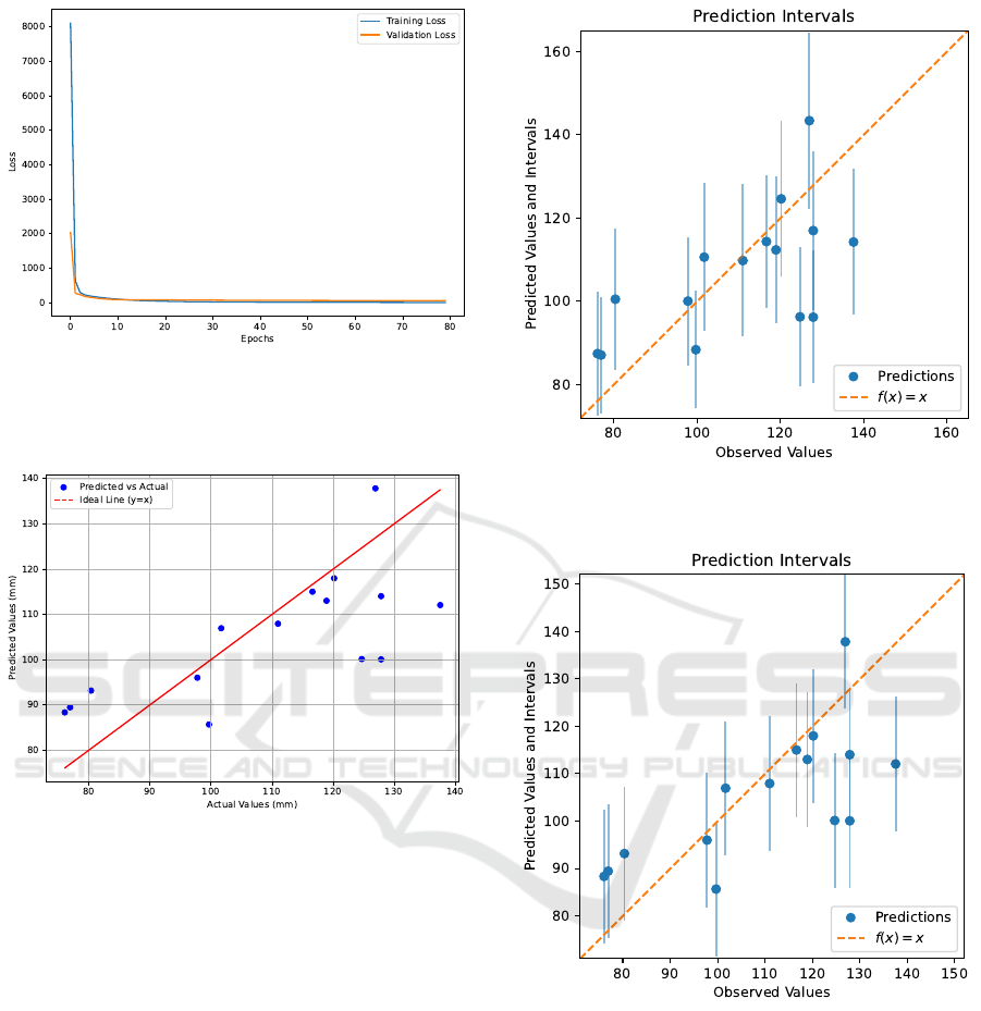
Figure 5: Training and validation loss throughout the entire

learning process. The ﬁnal model was obtained at epoch 75

using early stopping with a patience of 5, restoring the best

weights.

Figure 6: Actual values vs predicted values for the test set.

this strategy allowed us to isolate and assess the in-

dividual effects of key components: the backbone

network, data augmentation techniques, and model

head architecture without introducing excessive ex-

perimental complexity or confounding variables.

Table 2 presents the validation RMSE and R

for the different backbone networks we evaluated.

ViT-H/14 achieved the lowest validation RMSE and

the highest R

, signiﬁcantly outperforming the other

backbone networks. This indicates that ViT-H/14 is

highly recommended for this type of task. The ﬁne-

tuning results of the augmentation method, presented

in Table 3, show that the quality of the training dataset

and the use of systematic sampling are crucial factors

in few-shot learning. The results also highlight that

rotation, horizontal ﬂip, and brightness are the most

important parameters for improving the model’s gen-

eralization to real data.

Tables 4 and 5 summarize the hyperparameter tun-

ing conﬁgurations and outcomes for the model head

Figure 7: Uncertainty of predictions estimated by the MC

Dropout method for the test set.

Figure 8: Uncertainty of predictions estimated by the con-

formal prediction method for the test set.

architecture. They suggest the effect of the regression

head depth and the number of neurons in each layer

on the model’s performance.

In our current implementation, the ﬁnal output

layer employs a ReLU activation. While ReLU en-

forces non-negativity, which aligns with the positive

nature of lettuce width, it may also introduce an artiﬁ-

cial bias by truncating small predictions to zero. This

can be problematic in cases where the true value is

small but non-zero. A linear output layer could there-

fore be more appropriate, as it would preserve the

Uncertainty Estimation and Calibration of a Few-Shot Transfer Learning Model for Lettuce Phenotyping

393

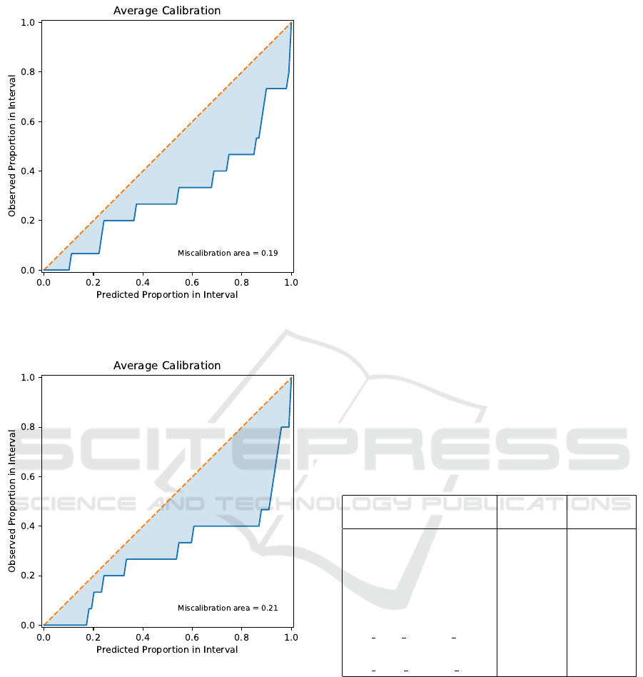
Figure 9: Calibration plot for uncertainty estimation using

the MC Dropout method.

Figure 10: Calibration plot for uncertainty estimation using

the “na

ıve” conformal prediction method.

continuous nature of the regression task without im-

posing unnecessary constraints. Future work may in-

vestigate this alternative to assess whether it improves

predictive accuracy.

While the above results are based on a single ran-

dom train–validation split, we further investigated the

robustness and generalizability of these ﬁndings by

repeating the experiments across 20 distinct random

splits. This enabled a statistical evaluation of perfor-

mance differences among backbone models, augmen-

tation strategies, and head architectures. Consistent

with the single-split results, ViT-H/14 again achieved

the lowest mean RMSE and the highest mean R

across all splits. Since the RMSE and R

distri-

butions did not satisfy normality or homogeneity of

variance assumptions, we applied the Kruskal–Wallis

test to assess statistical signiﬁcance. The analysis

showed that ViT-H/14 outperformed ResNet50, Efﬁ-

cientNetB0, ResNet101, and MobileNetV2 with sta-

tistically signiﬁcant differences at the 95% signiﬁ-

cance level.

For augmentation methods, horizontal ﬂip and

brightness yielded modest improvements compared

to the baseline, whereas rotation did not contribute

to performance gains. However, ANOVA tests on

the RMSE and R

distributions indicated that these

improvements were not statistically signiﬁcant at the

95% signiﬁcance level. Similarly, for model head

architectures, conﬁgurations with 512 and 128 neu-

rons in successive layers showed the best average per-

formance, but ANOVA suggested that these differ-

ences were also not statistically signiﬁcant. Taken to-

gether, these results suggest that while augmentation

and head depth exert some inﬂuence on performance,

the choice of backbone architecture remains the most

decisive factor for generalization in this setting.

Table 2: Comparison of different backbones using valida-

tion RMSE and R

. The Vision Transformer Huge with a

14×14 patch size achieves the lowest validation RMSE and

the highest R

Backbone Validation

RMSE

Validation

ResNet50 20.96 -0.4730

EfﬁcientNetB0 17.89 -0.0738

ResNet101 13.50 0.3886

MobileNetV2 15.79 0.1634

DenseNet121 14.94 0.2510

ViT

(vit base patch16 224)

15.77 0.1655

ViT

(vit huge patch14 224)

10.58 0.6244

In the transfer learning setup employed in this

study, the weights of the pretrained model were

frozen, and only a regression head was introduced at

the end of the backbone network for training. This

approach highlights the potential of backbone net-

works trained on large datasets for new tasks. A

further improvement would be ﬁne-tuning the back-

bone network by including its weights in the training

process. Our results suggest that transformer-based

architectures offer signiﬁcantly improved generaliza-

tion, with self-attention mechanisms capturing global

plant morphology more effectively than purely con-

volutional approaches.

KDIR 2025 - 17th International Conference on Knowledge Discovery and Information Retrieval

394

Table 3: Comparison of augmentation conﬁgurations used during hyperparameter tuning, evaluated using validation RMSE

and R

. Augmentations were implemented using torchvision transforms. Random rotations within a range of ±40

◦

, random

brightness adjustments within ±0.1, and random horizontal ﬂipping each sequentially improved performance on the validation

set.

Augmentation Technique Parameter Value Validation

RMSE

Validation R

No augmentation - - 10.58 0.6244

RandomRotation degrees

30° 9.38 0.7051

40° 8.80 0.7401

50° 8.98 0.7293

RandomHorizontalFlip p 0.5 8.35 0.7661

RandomVerticalFlip p 0.5 9.59 0.6914

ColorJitter brightness

0.1 7.61 0.8057

0.2 7.78 0.7967

RandomAfﬁne scale

(1, 1.1) 9.13 0.7202

(1, 1.2) 9.08 0.7232

(1, 1.3) 9.93 0.6694

RandomAfﬁne scale

(0.9, 1) 9.63 0.6888

(0.8, 1) 10.76 0.6118

RandomAfﬁne scale

(0.9, 1.1) 9.10 0.7225

(0.8, 1.2) 9.43 0.7020

RandomAfﬁne translate

0.1 9.89 0.6720

0.2 9.43 0.7020

0.3 9.80 0.6782

RandomAfﬁne shear

0.3 9.61 0.6901

10 8.64 0.7497

20 8.61 0.7516

Table 4: Effect of adding one layer. Comparison of the

number of neurons in the added layer using validation

RMSE and R

. Adding one layer did not result in improved

performance on the validation set.

Number of

neurons

Validation

RMSE

Validation R

512 7.78 0.7970

256 7.79 0.7963

128 7.86 0.7929

64 7.91 0.7903

Table 5: Effect of adding two layers. The second layer

was added after one layer with 512 neurons. Comparison

of the number of neurons in the second layer using valida-

tion RMSE and R

. Adding 32 neurons in the second layer

resulted in improved performance on the validation set.

Number of

neurons

Validation

RMSE

Validation R

256 8.31 0.7683

128 8.22 0.7736

64 8.11 0.7792

32 7.54 0.8094

16 7.88 0.7918

The learning curve (Figure 5 demonstrates a sharp

decline in both training and validation loss within the

initial epochs, indicating that the backbone network

had already learned most of the relevant information

in the input images. Consequently, the model re-

quired minimal additional learning, which it achieved

rapidly.

The dataset used in this study consisted of lettuce

samples with maximum widths ranging from 64.43

mm to 163.90 mm. Given this range, an RMSE of

14.34 mm indicated a promising model performance.

However, the R-squared value of 0.4464 suggests

that only 45% of the variance in the dependent vari-

able is explained by the model’s predictions. While

this level of accuracy may be sufﬁcient for growth

monitoring applications, it may not be acceptable in

more complex tasks where greater precision is re-

quired. Given the constraints of few-shot learning

due to the limited number of training images, this

performance can still be considered satisfactory, em-

phasizing the applicability of few-shot transfer learn-

ing in agricultural settings. Future work should ex-

plore other few-shot learning techniques, such as pro-

totypical networks (Snell et al., ), Siamese networks

(Koch et al., 2015), Model-Agnostic Meta-Learning

(MAML) (Finn et al., 2017), and MAML++ (Anto-

niou et al., 2018), to assess their performance on this

task.

Both MC dropout and conformal prediction

Uncertainty Estimation and Calibration of a Few-Shot Transfer Learning Model for Lettuce Phenotyping

395

proved to be effective and easily implementable meth-

ods for uncertainty estimation. The MC dropout

method requires the inclusion of dropout layers in the

network, whereas conformal prediction does not im-

pose such a requirement. In this regard, conformal

prediction offers a more ﬂexible and straightforward

implementation for any model.

As observed in Figure 7, the uncertainty estimated

by MC dropout remained relatively consistent across

all test dataset predictions, indicating that the model

maintains a uniform level of uncertainty across its

predictions. In contrast, the uncertainty estimated by

the ”Naive” CP method results in a ﬁxed-width inter-

val as shown in Figure 8. There remains a potential to

explore alternative variations of conformal prediction

methods beyond the ”Naive” approach, such as split

conformal prediction, to enhance uncertainty estima-

tion.

The calibration plots for both methods given in

Figs. 9 and 10 indicate that the miscalibration area

is relatively low, suggesting that the model exhibits

some degree of calibration. However, there remains

room for further calibration improvement. The mis-

calibration area (0.19) for the Monte Carlo (MC)

dropout method was slightly smaller compared to the

conformal prediction method (0.21). MC dropout

method had empirical coverage of 73% at the nominal

90% and 95% conﬁdence levels. In contrast, confor-

mal prediction method had empirical coverages 47%

and 80% at the nominal 90% and 95% conﬁdence lev-

els. This further showed that the MC dropout method

resulted in better calibration in uncertainty estimation

compared to conformal prediction method in this task.

To further improve the calibration of the uncertainty

estimates produced by the MC Dropout method, iso-

tonic regression (Jiang et al., 2011) was employed us-

ing the validation set. However, this resulted in no

improvement, which could be attributed to the limited

amount of data.

6 CONCLUSION

In conclusion, the study demonstrates that our

pipeline: few-shot transfer learning, combined with

techniques such as MC dropout and conformal pre-

diction, can be effectively applied to agricultural tasks

such as lettuce growth monitoring and quantify as-

sociated uncertainties, even when trained on lim-

ited data. While the model performed promisingly

with the limited data, there are still opportunities to

improve accuracy, calibration, and uncertainty esti-

mation. Incorporating uncertainty quantiﬁcation not

only improves conﬁdence in predictions but also sup-

ports safer deployment in agricultural environments,

where decisions informed by reliable model outputs

are critical.

ACKNOWLEDGEMENTS

We would like to acknowledge the ﬁnancial support

from the Research Council of Norway (project num-

ber 354125) and Photosynthetic AS. We also wish to

thank the Norwegian University of Life Sciences for

granting admission.

REFERENCES

Antoniou, A., Edwards, H., and Storkey, A. (2018). How to

train your maml. arXiv, 1810.09502.

Belissent, N., Pe

na, J. M., Mes

ıas-Ruiz, G. A., Shawe-

Taylor, J., and P

erez-Ortiz, M. (2024). Transfer and

zero-shot learning for scalable weed detection and

classiﬁcation in uav images. Knowledge-Based Sys-

tems, 292:111586.

Chang, L. and Lin, Y.-H. (2025). Few-shot remaining useful

life prediction based on bayesian meta-learning with

predictive uncertainty calibration. Engineering Appli-

cations of Artiﬁcial Intelligence, 142:109980.

Chollet, F. et al. (2015). Keras. https://keras.io.

Deng, J., Dong, W., Socher, R., Li, L.-J., Li, K., and Fei-

Fei, L. (2009). Imagenet: A large-scale hierarchical

image database. In 2009 IEEE Conference on Com-

puter Vision and Pattern Recognition, pages 248–255.

Ding, P., Jia, M., Ding, Y., Cao, Y., Zhuang, J., and Zhao,

X. (2023). Machinery probabilistic few-shot prognos-

tics considering prediction uncertainty. IEEE/ASME

Transactions on Mechatronics, 29(1):106–118.

Dutta, A. and Zisserman, A. (2019). The VIA annotation

software for images, audio and video. In Proceedings

of the 27th ACM International Conference on Multi-

media, MM ’19, New York, NY, USA. ACM.

Finn, C., Abbeel, P., and Levine, S. (2017). Model-agnostic

meta-learning for fast adaptation of deep networks. In

International conference on machine learning, pages

1126–1135. PMLR.

Gal, Y. and Ghahramani, Z. (2016). Dropout as a bayesian

approximation: Representing model uncertainty in

deep learning. In Balcan, M. F. and Weinberger,

K. Q., editors, Proceedings of The 33rd International

Conference on Machine Learning, volume 48 of Pro-

ceedings of Machine Learning Research, pages 1050–

1059, New York, New York, USA. PMLR.

He, J., Zhang, X., Lei, S., Alhamadani, A., Chen, F., Xiao,

B., and Lu, C.-T. (2023). Clur: uncertainty estima-

tion for few-shot text classiﬁcation with contrastive

learning. In Proceedings of the 29th ACM SIGKDD

Conference on Knowledge Discovery and Data Min-

ing, pages 698–710.

KDIR 2025 - 17th International Conference on Knowledge Discovery and Information Retrieval

396

Hossen, M. I., Awrangjeb, M., Pan, S., and Mamun, A. A.

(2025). Transfer learning in agriculture: a review. Ar-

tiﬁcial Intelligence Review, 58(4):97.

ullermeier, E. and Waegeman, W. (2021). Aleatoric and

epistemic uncertainty in machine learning: An intro-

duction to concepts and methods. Machine learning,

110(3):457–506.

Iwata, T. and Kumagai, A. (2023). Meta-learning to cali-

brate gaussian processes with deep kernels for regres-

sion uncertainty estimation. arXiv, 2312.07952.

Jiang, X., Osl, M., Kim, J., and Ohno-Machado, L. (2011).

Smooth isotonic regression: a new method to calibrate

predictive models. AMIA Summits on Translational

Science Proceedings, 2011:16.

Kendall, A. and Gal, Y. (2017). What uncertainties do we

need in bayesian deep learning for computer vision?

Advances in neural information processing systems,

30.

Kingma, D. P. and Ba, J. (2014). Adam: A method for

stochastic optimization. arXiv, 1412.6980.

Koch, G., Zemel, R., Salakhutdinov, R., et al. (2015).

Siamese neural networks for one-shot image recog-

nition. In ICML deep learning workshop, volume 2,

pages 1–30. Lille.

Lagergren, J., Pavicic, M., Chhetri, H. B., York, L. M., Hy-

att, D., Kainer, D., Rutter, E. M., Flores, K., Bailey-

Bale, J., Klein, M., et al. (2023). Few-shot learning

enables population-scale analysis of leaf traits in pop-

ulus trichocarpa. Plant Phenomics, 5:0072.

Luo, J., Li, B., and Leung, C. (2023). A survey of com-

puter vision technologies in urban and controlled-

environment agriculture. ACM Computing Surveys,

56(5):1–39.

Mokhtar, A., El-Ssawy, W., He, H., Al-Anasari, N., Sam-

men, S. S., Gyasi-Agyei, Y., and Abuarab, M. (2022).

Using machine learning models to predict hydroponi-

cally grown lettuce yield. Frontiers in Plant Science,

13:706042.

Morales-

Alvarez, P., Christodoulidis, S., Vakalopoulou, M.,

Piantanida, P., and Dolz, J. (2024). Bayesadapter: en-

hanced uncertainty estimation in clip few-shot adapta-

tion. arXiv, 2412.09718.

Ojo, M. O. and Zahid, A. (2022). Deep learning in con-

trolled environment agriculture: A review of recent

advancements, challenges and prospects.

Park, S., Cohen, K. M., and Simeone, O. (2023). Few-shot

calibration of set predictors via meta-learned cross-

validation-based conformal prediction. IEEE Trans-

actions on Pattern Analysis and Machine Intelligence,

46(1):280–291.

Ruan, S., Cang, H., Chen, H., Yan, T., Tan, F., Zhang, Y.,

Duan, L., Xing, P., Guo, L., Gao, P., et al. (2023).

Hyperspectral classiﬁcation of frost damage stress in

tomato plants based on few-shot learning. Agronomy,

13(9):2348.

Snell, J., Swersky, K., and Zemel, T. R. Prototypical net-

works for few-shot learning.

Tibshirani, R. (2023). Conformal prediction.

Wang, D., Cao, W., Zhang, F., Li, Z., Xu, S., and Wu, X.

(2022a). A review of deep learning in multiscale agri-

cultural sensing. Remote Sensing, 14(3):559.

Wang, X., Vladislav, Z., Viktor, O., Wu, Z., and Zhao, M.

(2022b). Online recognition and yield estimation of

tomato in plant factory based on yolov3. Scientiﬁc

Reports, 12(1):8686.

Wightman, R. (2019). Pytorch image models. https:

//github.com/rwightman/pytorch-image-models.

Yang, J., Guo, X., Li, Y., Marinello, F., Ercisli, S., and

Zhang, Z. (2022). A survey of few-shot learning

in smart agriculture: developments, applications, and

challenges.

Zhang, P. and Li, D. (2022). Yolo-volo-ls: a novel method

for variety identiﬁcation of early lettuce seedlings.

Frontiers in plant science, 13:806878.

Uncertainty Estimation and Calibration of a Few-Shot Transfer Learning Model for Lettuce Phenotyping

397