Optimizing Sensor Deployment Strategy for Tracking Mobile Heat
Source Trajectory
Thanh Phong Tran
1 a
, Laetitia Perez
2 b
, Laurent Autrique
2 c
, Edouard Leclercq
1 d
,
Syrine Bouazza
1 e
and Dimitri Lefevbre
1 f
1
GREAH, Universit
´
e Le Havre Normandie, 25 Street Philippe Lebon, Le Havre, France
2
LARIS, University of Angers, 62 Av. Notre Dame du Lac, Angers, France
Keywords:
Inverse Problem, Moving Heat Source, Optimal Assignment Problem, Partial Differential Equation,
Parametric Identification.
Abstract:
Previous studies have investigated inverse problems in physical systems described by partial differential equa-
tions, particularly for identifying unknown parameters of mobile heat sources. An iterative minimization of a
quadratic cost function, based on the conjugate gradient method, has shown reliable results in identifying heat
densities and trajectories both offline and online. Although fixed sensor arrays can be effective, covering the
full operating range of a moving heat source requires a large number of sensors, leading to inefficiencies and
waste. A more efficient approach uses fewer mobile sensors mounted on autonomous robots. However, this
introduces challenges in robot control, ensuring optimal positioning, coordination, and collision avoidance.
To address this, we propose a method that combines sensitivity-based sensor placement with robot assignment
algorithms such as the Hungarian Algorithm and Multi-Agent Path Finding. This enables effective tracking
of the heat source’s trajectory while optimizing sensor deployment. The approach not only increases overall
sensitivity of the sensor network but also improves identification performance with reduced latency and higher
accuracy.
NOMENCLATURE
c specific heat capacity, Jkg
−1
K
−1
s
i
(t) basis function for piecewise linear functions
s(t) vector of basis function s
i
(t)
t,t
f
time and final time, s
t
id
identification time, s
t
d
delay time, s
x(t),y(t) space variable, m
x(t),y(t) vector related to space variable, m
σ
res
standard deviation of temperature residual, K
σ
δd
standard deviation of trajectory estimation, m
µ
delay
average delay on the identification, s
µ
res
average temperature residual, K
µ
δd
average trajectory estimation errors, m
a
https://orcid.org/0000-0002-5596-8524
b
https://orcid.org/0000-0001-6340-0317
c
https://orcid.org/0000-0002-7611-4923
d
https://orcid.org/0000-0003-2840-1378
e
https://orcid.org/0000-0001-5040-3690
f
https://orcid.org/0000-0001-7060-756X
φ(t) heat flux density, W m
−2
φ(t) vector related to heat flux density, W m
−2
η precision of heat flux discontinuity
λ thermal conductivity, W m
−1
K
−1
ρ la masse volumique, kgm
−3
θ temperature, K
h heat transfer coefficient, Jkg
−1
K
−1
e plate thickness, m
l plate dimension (width, length), m
−→
n unit external outward-pointing vector
n number of robot-sensors
N number of time interval for identification
N
vs
number of virtual sensors
N
t
number of identification resolution
r heat flux radius, m
τ related to time discretization, s
Tran, T. P., Perez, L., Autrique, L., Leclercq, E., Bouazza, S. and Lefevbre, D.
Optimizing Sensor Deployment Strategy for Tracking Mobile Heat Source Trajectory.
DOI: 10.5220/0013742600003982
Paper published under CC license (CC BY-NC-ND 4.0)
In Proceedings of the 22nd International Conference on Informatics in Control, Automation and Robotics (ICINCO 2025) - Volume 1, pages 477-485
ISBN: 978-989-758-770-2; ISSN: 2184-2809
Proceedings Copyright © 2025 by SCITEPRESS – Science and Technology Publications, Lda.
477

1 INTRODUCTION
In recent years, the study of partial differential equa-
tions (PDEs) has received increasing attention, sup-
ported by advances in computational tools and pow-
erful computing systems. PDEs play a crucial role
across a wide range of fields, from military ap-
plications (such as aerospace and national security)
to science and daily life, including physics, biol-
ogy, finance, and engineering. Researchers have in-
creasingly focused on modeling complex problems
and phenomena using systems of linear or nonlinear,
single-order or higher-order PDEs, and on develop-
ing methods to solve them effectively (Hussein and
Rusul, 2020). Moreover, the solution of inverse prob-
lems related to PDEs has become a growing area of
interest, as it often requires sophisticated techniques,
including both classical mathematical approaches and
modern methods involving artificial intelligence and
machine learning (Berg and Nystr
¨
om, 2021; Aarset
et al., 2023).
In the course of researching methods to identify
the parameters of mobile heat sources, specifically
heat density and movement trajectory, the authors
have developed an identification approach that com-
bines the Gradient Conjugate Method (GCM) with an
iterative procedure. This approach is based on min-
imizing a cost function derived from the comparison
between temperature data collected by thermal sen-
sors and data generated from theoretical models. This
inverse heat conduction problem-solving framework
is well-known as ill-posed in the Hadamard sense,
based on the GCM involves three key components:
the direct problem, the adjoint problem, and the sen-
sitivity problem (Fakih et al., 2024). The authors have
successfully performed both offline and online iden-
tification of the heating flux or the trajectory, as well
as simultaneous identification of both parameters for
one or multiple heat sources, whether fixed or mobile.
The identification algorithms employ iterative meth-
ods using sliding windows, either with fixed size or
adaptively adjusted, in combination with future value
prediction techniques.
The proposed thermal sensor configurations in-
clude both fixed and mobile sensors, the latter being
deployed on autonomous robots. Notably, the selec-
tion and control of mobile sensors have been identi-
fied as critical factors that significantly influence the
efficiency of the parameter identification process in
terms of accuracy, computational cost, and response
delay. Over the years, the authors have developed
methods for determining optimal sensor location and
selection strategies for mobile robots based on the
sensitivity problem. The robot navigation strategies
proposed so far are heuristic, in which robots priori-
tize tasks and move toward the nearest target location
(Chakraa et al., 2023; Chakraa et al., 2025). However,
the collision problem is not addressed in this paper but
will be in future work.
This paper is structured into the following four
parts. The first part will briefly present the research
problem and the context of the physical system in
which the mathematical modeling of the direct prob-
lem and the formulation of the inverse problem, ded-
icated to identifying the trajectory of a moving heat
source will be presented. In the second part, the
methodology of quasi-online identification using a
method of selecting sensor positions based on sensi-
tivity problem combined with strategy for deploying
sensor network will be presented. The numerical re-
sults will be considered to discuss strategies for de-
ploying the sensor network in Section 4. The last sec-
tion will represent concluding remarks of this study.
2 MODELING AND INVERSE
PROBLEM FORMULATION
2.1 Physical System Presentation
The heat conduction equation is a partial differential
equation that describes the distribution of heat in a
given object over time. Once this temperature dis-
tribution is known, the conductive heat flux at any
point in the material or on its surface can be calcu-
lated using Fourier law. The general form of the 3D
heat conduction equation describes how temperature
varies in a three-dimensional space over time. The
general equation is:
ρC
∂θ(x,y,z,t)
∂t
− λ∆θ(x,y,z,t) = Q (x, y,z,t) (1)
where Q(x,y,z,t) is the internal heat generation per
unit volume (W /m
3
), and ∆ is Laplace operation, see
Eq. 4. This mathematical model of the diffusion
equation in three-dimensional (Eq. 1) can be reduced
into a similar two-dimensional pattern (Eq. 6) within
certain limits that did not change the physical proper-
ties of heat transfer process (Tran, 2018a). From now
on, the temperature as a function of space and time
will be denoted by θ(x,y,t) and expressed in Kelvin
(K).
In this study, a mobile heat source is modeled as
a disk which moves along a trajectory S on a square
aluminum plate with dimensions Ω = L ×L ×e ⊂ R
3
,
where L represents the side length and e the thickness.
The boundary of this domain is denoted ∂Ω ⊂ R
2
.
Spatial coordinates within the reduced 2D domain are
ICINCO 2025 - 22nd International Conference on Informatics in Control, Automation and Robotics
478

X
-0.5 -0.4 -0.3 -0.2 -0.1 0 0.1 0.2 0.3 0.4 0.5
Y
-0.5
-0.4
-0.3
-0.2
-0.1
0
0.1
0.2
0.3
0.4
0.5
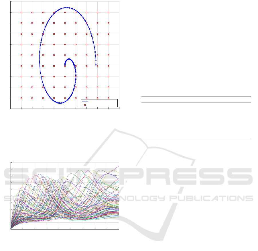
Real source's trajectory
Virtual sensor position
Figure 1: Heat source trajectory and mesh of sensors.
given by (x, y) ⊂ ]−L/2,L/2[ in meters, while the
temporal variable t belongs to the interval T = [0,t
f
],
where t
f
marks the final observation time, expressed
in seconds.
Time (s)
0 200 400 600 800 1000 1200 1400 1600 1800
Temperature of virtual sensor (°C)
0
20
40
60
80
100
120
140
160
180
200
Figure 2: Time and spatial temperature evolution.
For this moving heat source, we apply a time-
dependent heat density flux φ(t) (in Wm
−2
) to the sur-
face of the plate. This density flux is concentrated
over a fixed, homogeneous circular area D of radius
r, centered at the point I(x
I
(t), y
I
(t))(Tran, 2018b).
Heat source total heating flux is defined by:
Φ(x,y,t) =

φ(t) if (x, y) ∈ D (I(t),r)
0 otherwise
(2)
and could be expressed continuously and differen-
tiably as in Eq. 5 (see Table 2), where the param-
eter η ∈ R
+
is related to the heat flux discontinu-
ity at the disk boundary. Without loss of general-
ity, the time interval T = [0,t
f
] =
N
t
−1
∪
d=0
[t
d
,t
d+1
] is di-
vided into N
t
segments, with t
d
= τd and τ = t
f
/N
t
.
Thus, the coordinates of trajectory are discretized as
x(t) =
∑
x
d
s
d
(t), y(t) =
∑
y
d
s
d
(t), and then x
d
= x(t
d
),
y
d
= y(t
d
). The basis of hat functions for time dis-
cretization is ∀d = 0, ..., N
t−1
:
s
d
(t) =



1 +t/τ − d if t ∈ [t
d−1
,t
d
]
1 −t/τ + d if t ∈ [t
d
,t
d+1
]
0 otherwise
(3)
The temperature evolution of virtual sensors on the
alunimium will be represented in Fig. 2. The numeri-
cal solution of system (Eq. 6) can be achieved by im-
plementing the finite element method of Comsol Mul-
tiphysics interfaced with Matlab using parameters in
Table 1.
Table 1: Value of input parameters.
Symbol, Definition Value
Volumetric heat capacity, ρC 2.421e6 J/(m
3
K)
Natural convection, h 10 W/(m
2
K)
Thermal conductivity, λ 237 W/(m
2
K)
Initial temperature, θ
0
294.15K
Final time, t
f
1800 s
Thickness, e 2e−3 m
2.2 Inverse Problem Formulation
In order to identify the trajectory I(x
I
(t), y
I
(t)) of the
mobile heat source from the measured temperature
changes using n sensors on the plate, an inverse prob-
lem can be formulated and solved by minimizing a
quadratic criterion (Eq. 7).
An iterative conjugate gradient regularization
method was implemented to identify unknown pa-
rameters (Tran et al., 2017; Vergnaud et al., 2015;
Tran, 2018b; Fakih et al., 2024). The algorithm of
this method consists of iteratively solving three well-
posed problems in the Hadamard sense: direct prob-
lem, adjoint problem, and sensitivity problem.
• A direct problem (Eq. 6) gives the spatio-
temporal evolution of temperature θ(x,y,t) to cal-
culate the criterion J(θ,Φ) (see Eq. 7), so that it
helps to judge the quality of the estimates at itera-
tion k by using this stop condition J(θ,Φ) < J
stop
.
• An adjoint problem (Eq. 8) gives the spatio-
temporal evolution of temperature adjoin function
ψ(x,y,t) to calculate the cost function gradients
by unknown parameters
−→
∇J(θ,x
k
) and
−→
∇J(θ,y
k
)
(see Eq. 9), then to define the descent direction of
unknown parameters
−→
d
k+1
x
and
−→
d
k+1
y
(Eq. 10).
• A sensitivity problem (Eq. 11) gives the spatio-
temporal evolution of variation of temperature
δθ(x,y,t) to calculate the descent depth γ
k+1
(Eq.
12) in the descent direction.
Optimizing Sensor Deployment Strategy for Tracking Mobile Heat Source Trajectory
479

Table 2: Literature of models/equations for unknown parameter identification based on CGM.
As presented in (Beddiaf et al., 2012; Beddiaf et al., 2014; Fakih et al., 2024)
1. Laplace operator
∆θ(x,y,t) =
∂
2
θ(x,y,t)
∂x
2
+
∂
2
θ(x,y,t)
∂y
2
+
∂
2
θ(x,y,t)
∂z
2
(4)
2. Total heat flux
Φ(x,y,t) =
φ(t)
π
arccot

η
q
(x − x
I
(t))
2
+ (y − y
I
(t))
2
− r

(5)
As presented in (Tran et al., 2017; Tran, 2018b; Vergnaud et al., 2014; Vergnaud et al., 2015; Vergnaud
et al., 2016; Vergnaud et al., 2020; Fakih et al., 2024)
3. Direct problem











ρC
∂θ(x,y,t)
∂t
− λ∆θ(x,y,t) =
Φ(x,y,t) − 2h(θ(x, y,t) − θ
0
)
e
on Ω × T
θ(x,y,0) = θ
0
(x,y) on Ω
− λ
∂θ(x,y,t)
∂⃗n
= 0 on ∂Ω × T
(6)
4. Cost function
J(θ,Φ) =
1
2
Z
T
N
c
∑
n=1

θ(C
n
,t,Φ) −
ˆ
θ(C
n
,t)

2
dt at sensors C
n
(7)
5. Adjoint problem











ρC
∂ψ(x,y,t)
∂t
− λ∆ψ(x,y,t) = E(x, y,t) +
2hψ(x,y,t)
e
on Ω × T
ψ(x,y,t
f
) = 0 on Ω
− λ
∂ψ(x,y,t)
∂⃗n
= 0 on ∂Ω × T
(8)
6. Gradient of unknown parameters (where ω(x, y,t) =
p
(x − x
I
(t))
2
+ (y − y
I
(t))
2
)
−→
∇J(θ, x
k
) = −
t
f
Z
0
Z
Ω
µφ(t)
π
·
(x − x
I
(t))
ω(x,y,t) (1 +µ
2
(ω(x,y,t) − r)
2
)
· s
d
x
(t) ·
ψ(x,y,t)
e
dΩ dt (a)
−→
∇J(θ, y
k
) = −
t
f
Z
0
Z
Ω
µφ(t)
π
·
(y − y
I
(t))
ω(x,y,t) (1 +µ
2
(ω(x,y,t) − r)
2
)
· s
d
y
(t) ·
ψ(x,y,t)
e
dΩ dt (b)
(9)
7. Descent direction
−→
d
k+1
x
= −
−→
∇J(θ, x
k
) +



−→
∇J(θ, x
k
)



2



−→
∇J(θ, x
k−1
)



2
−→
d
k
x
and
−→
d
k+1
y
= −
−→
∇J(θ, y
k
) +



−→
∇J(θ, y
k
)



2



−→
∇J(θ, y
k−1
)



2
−→
d
k
y
(10)
8. Sensitivity problem











ρC
∂δθ(x,y,t)
∂t
− λ∆δθ(x,y,t) =
δΦ(x,y,t) − 2hδθ(x,y,t)
e
on Ω × T
δθ(x,y,0) = 0 on Ω
− λ
∂δθ(x,y,t)
∂⃗n
= 0 on ∂Ω × T
(11)
9. Descent depth
γ
k+1
=
Z
T
N
c
∑
n=1

θ(C
n
,t,
−→
Φ
k
) −
ˆ
θ(C
n
,t)

δθ(C
n
,t,
−→
Φ
k
)dt
Z
T
N
c
∑
n=1
δθ(C
n
,t,
−→
Φ
k
)
2
dt
(12)
10. Updating new value
x
k+1
= x
k
− γ
k+1
d
k+1
x
, and y
k+1
= y
k
− γ
k+1
d
k+1
y
(13)
ICINCO 2025 - 22nd International Conference on Informatics in Control, Automation and Robotics
480

The key challenges in tracking mobile heat source
are accurately determining the locations of the sensors
to collect precise and sensitive temperature data, and
developing an efficient strategy for moving the robot-
sensors to ensure timely data acquisition. Algorithm
1 allows us to select the most relevant positions to
move n robot-sensors c
i=1,2,...,n
whose over the time
interval τ
m
= [τ
−
m
,τ
+
m
] by maximizing the Euclidean
norm of temperature variation L
2
i
=


δθ

c
i
,t



(see,
Eq. 14) over sliding time intervals τ
m
(Tran, 2018b).
This algorithm returns a list of goal positions G for
the robot-sensors.
Algorithm 1: Method for selecting the sensor’s next posi-
tions.
Data: initialisation n, L
2
, τ
m
← [τ
−
m
,τ
+
m
]
Result: calculate the most sensible positions;
solve sensitivity problem δθ(c
i
,t)
calculate Euclidean norm L
2
i
L
2
i
=
s
∑
τ
m
(δθ(c
i
,t))
2
∀i = 1,2,.. .,N
vs
(14)
while i < n;
do
choose a sensor c
i
of the largest value of
L
2
i
;
G ← G + c
i
remove this sensor i in the list
i ← i + 1
return G (List of goal positions).
end
Next, we study how to assign the computational
positions to the n robot-sensors. To do this, we solve
a Linear Assignment Problem (LAP) using the Hun-
garian algorithm (Chakraa et al., 2025; Rinaldi et al.,
2024; Chopra et al., 2017; Ismail and Sun, 2017)
which will be introduced in the next section. The task
now is to find the optimal solution to deploy the robots
(called the mobile sensor network) from their current
positions in R to the goal positions in G.
3 DEPLOYING SENSOR
NETWORK STRATEGY
3.1 Problem Statement
In multi-robot mobility systems, efficiently allocat-
ing the movement sequence of each robot in the
group plays an important role in minimizing the total
amount of resources used, such as energy consump-
tion or travel time to the destination (Zhang et al.,
2023; Luo et al., 2023; Smith and Jones, 2023; Doe
and Roe, 2025). In this paper, we propose an algo-
rithm to solve the problem of optimally assigning n
mobile robots to n predefined target locations so that
the total travel distance is minimized. Each set of cur-
rent positions of the robots and the set of targets are
represented as position coordinates in a 2D Cartesian
plane. The cost of assigning a given robot to a tar-
get is defined as the Euclidean distance between their
corresponding coordinates.
3.2 Mathematical Formulation of
Assignment Algorithm
Let R = {r
1
(x
r
1
,y
r
1
),r
2
(x
r
2
,y
r
2
),.. .,r
n
(x
r
n
,y
r
n
)}
denote the set of robots; G =
{g
1
(x
g
1
,y
g
1
),g
2
(x
g
2
,y
g
2
),.. .,g
n
(x
g
n
,y
g
n
)} denote the
set of goals. And, let d
i j
be the cost (distance) for
robot i to reach goal position j, defined as:
d
i j
=
q
(x
r
i
− x
g
j
)
2
+ (y
r
i
− y
g
j
)
2
(15)
The binary decision variable b
i j
∈ {0,1} is defined by
:
b
i j
=
(
1 if robot i is assigned to goal j
0 otherwise
(16)
The applied objective of the LAP algorithm is to as-
sign n robots to n goals in a way that minimizes the
total assignment cost. The mathematical formulation
of the LAP is given as follows:
f = min
n
∑
i=1
n
∑
j=1
d
i j
· b
i j
(17)
The constraints presented in (18) guarantee a one-to-
one correspondence between robots and goals, such
that each robot is assigned to exactly one goal and
vice versa.
n
∑
j=1
b
i j
= 1, and
n
∑
i=1
b
i j
= 1 ∀i, j ∈ {1,2,. ..,n}
(18)
In previous studies, we have successfully demon-
strated the identification of the heating flux and the
moving trajectory of the heat source with various sen-
sor configurations (from 1 to 9 sensors and more).
These studies have shown that the smaller the number
of sensors (e.g. n = 1), the less the observed data has
been and the poor accuracy has been achieved. On the
contrary, the larger the number of sensors (e.g. n = 9
and more), the larger the collected data set will be,
Optimizing Sensor Deployment Strategy for Tracking Mobile Heat Source Trajectory
481

including unreliable noisy data, making the compu-
tation time important and even affecting the accuracy.
Particularly for mobile sensor systems, the smaller the
number of sensors, the easier it will be to manage and
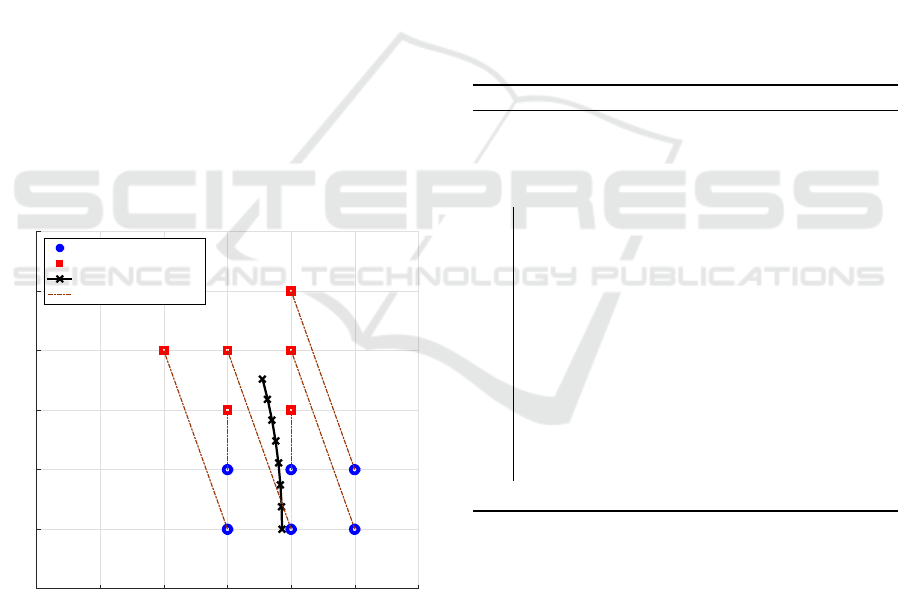
control. In this study, we illustrate the method with n
= 6 robot-sensors as an example. Consider the set of
robot-sensor current positions R={(0.2,-0.1), (0.2,0),
(0.3,-0.1), (0.3,0), (0.4,-0.1), (0.4,0)} and the set of
robot-sensor next positions G = {(0.3,0.1), (0.2,0.2),
(0.3,0.2), (0.2,0.1), (0.3,0.3), (0.1,0.2)} (Fig. 3). The
cost matrix is calculated using the Euclidean distance
(Eq. 15) and gives the following result:
D =







0.224 0.300 0.316 0.200 0.412 0.316
0.141 0.200 0.224 0.100 0.316 0.224
0.200 0.316 0.300 0.224 0.400 0.361
0.100 0.224 0.200 0.141 0.300 0.283
0.224 0.361 0.316 0.283 0.412 0.424
0.141 0.283 0.224 0.224 0.316 0.361







The optimal assignment is obtained by solving
the above LAP using the Hungarian algorithm, also
known as the Kuhn-Munkres algorithm. This algo-
rithm efficiently finds a minimum-cost (Eq. 17) per-
fect matching in a weighted bipartite graph and runs
in O(n
3
) time (Giordani et al., 2010). It ensures opti-
mal solutions by continuously improving feasible la-
bels and enhancing paths.
-0.1 0 0.1 0.2 0.3 0.4 0.5
-0.2
-0.1
0
0.1
0.2
0.3
0.4
R1
R2
R3
R4
R5
R6
G1
G2 G3
G4
G5
G6
Robot's current positions
Robot's next positions
Source trajectory
Assignments
Figure 3: Presentation of LAP using the Hungarian algo-
rithm.
This provides an optimal solution for assigning
robot-sensor next positions to robots in scenarios
where the costs are additive and independent. In
Fig. 3, Robot 1 moves to position 6, and respectively
Robot 2 moves to position 4, Robot 3 moves to posi-
tion 2, Robot 4 moves to position 1, Robot 5 moves
to position 3, and Robot 6 moves to position 5. The
total calculated cost is 1.46. In this study, it is as-
sumed that the robot-sensors move at the same speed
and have the same accuracy. The above results show
that the robot-sensors have different travel distances,
so the travel time to the required locations is also dif-
ferent. Therefore, the priority order is that the robots
that need to travel far will start first.
Accordingly, the problem of trajectory collisions
needs to be considered in practice in order to ensure
that multiple agents can avoid one another. Future
work will focus on addressing this issue. This paper
is limited to calculating the optimal travel distance.
3.3 Sensor Assignment Problem
A strategy for deploying sensor network using the
LAP was proposed and applied to control the move-
ment of n robot-sensors to measure the temperature in
order to identify the moving trajectory of the mobile
heat source. This deployment strategy is introduced
in Algorithm 2.
Algorithm 2: Deploying sensor network method for CGM.
Data: initialisation: R, G, τ
m
= [τ
−
m
,τ
+
m
]
Result: estimate the trajectory ˆx
I
(t), ˆy
I
(t)
while J(θ, Φ) < J
stop
;
do
apply Algorithm 1:
G ← G + c
i
;
calculate Euclidean norm of cost matrix:
D ← d
i j
;
apply algorithm LAP:
G
j
← R
i
;
deploy robot-sensors from set of R to G ;
collect temperature data:
ˆ
θ(x,y,t) ;
apply identification based on CGM:
( ˆx
I
(t), ˆy
I
(t)) ;
load next time interval: τ
m
← τ
m+1
;
return ˆx
I
(t), ˆy
I
(t)
end
The next positions of the robot-sensors are calcu-
lated by Algorithm 1. Next, the cost matrix is calcu-
lated by combining the distances between the robots
of R and the next positions G based on the Euclidean
norm and applying the LAP algorithm to find the op-
timal positions and assign each robot-sensor R
i
to the
best next position G
j
such that the total cost is min-
imized. When the robots reach to positions G, they
will collect temperature data
ˆ
θ(x,y,t) and send them
to the CGM algorithm to estimate current positions of
the heat source. Finally, the algorithm will repeat the
determination of the robot position for the next time
interval.
ICINCO 2025 - 22nd International Conference on Informatics in Control, Automation and Robotics
482

4 NUMERICAL RESULTS AND
DISCUSSION
This section presents numerical results to evaluate
proposed algorithms (for selecting the sensor posi-
tions using the sensitivity problem, and for deploying
the sensor network using LAP) and method of identi-
fication based on CGM for determining the unknown
trajectory of a single moving heat source. The ob-
jective is to minimize the output error by accurately
estimating the trajectory of the heat source. The data
set of temperature within the domain is a solution of
the system of PDEs and is thus the acquisition of mea-
surements by sensors. The temperatures are noisy and
distributed by a normal distribution N(µ, σ) to reflect
actual measurement conditions.
X
-0.5 -0.4 -0.3 -0.2 -0.1 0 0.1 0.2 0.3 0.4 0.5
Y
-0.5
-0.4
-0.3
-0.2
-0.1
0
0.1
0.2
0.3
0.4
0.5
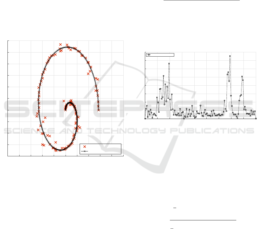
Estimated trajectory
Real trajectory
Figure 4: Presentation of estimated trajectory using the Gra-
dient Conjugate Method.
The numerical results which were obtained by im-
plementing the finite element method of Comsol Mul-
tiphysics 3.5 interfaced with Matlab R2012b, were
performed on a personal computer with the following
configuration: CPU Intel® Core™ i7-3520M CPU @
2.90GHz, RAM 8.00 GB, OS Windows 11 (64-bit).
These results demonstrate the implementation of the
CGM in solving the inverse problem of determining
the trajectory of a moving heat source I(x
I
(t), y
I
(t)),
according to the defined stopping criterion. Accord-
ingly, the trajectory of the studied source is deter-
mined after an identification time t
id
= 1, 887s. The
numerical experimental time is 30 minutes. The
final estimate of the trajectory of the heat source
ˆ
I( ˆx
I
(t), ˆy
I
(t)) is shown in Figure 4.
In order to estimate the trajectory identification
quality, we calculate the average of the temperature
residual µ
res
, the standard deviation of temperature
residual σ
res
, the average of the trajectory error µ
δd
,
the standard deviation of the trajectory error σ
δd
and
the maximum max
δd
of errors between estimated and
real heat source trajectory considering a Gaussian
noise N(0, 1) with mean µ = 0 and standard deviation
σ = 1 on measured temperature.
The error of the trajectory estimation is calculated
using Eq. 19:
δd =
q

x
I
(t) − ˆx
I
(t)

2
+

y
I
(t) − ˆy
I
(t)

2
(19)
The position errors of the identified trajectory com-
pared to the real trajectory of the moving heat source
are calculated and shown as Figure 5. Accordingly,
the largest position error value is max
δd
= 3.767 ×
10
−2
m.
Time (s)
0 200 400 600 800 1000 1200 1400 1600 1800
Range of trajectory errors (m)
0
0.005
0.01
0.015
0.02
0.025
0.03
0.035
0.04
Source's trajectory errors
Figure 5: Presentation of trajectory estimation errors
As observed in Figure 5, the trajectory error ex-
hibits notable peaks, particularly around the time
points of 400 s and 1400 s. These fluctuations may be
attributed to disturbances in the sensor network, espe-
cially when the next positions of the sensors are not
accurately determined. These issues should be further
investigated and addressed in future studies.
The average and the standard deviation of temper-
ature residual are determined by:
µ
res
=
1
n
n
∑
i=1

θ(x,y,t, I) −
ˆ
θ(x,y,t)

(20)
σ
res
=
s
1
n
n
∑
i=1

θ(x,y,t, I) −
ˆ
θ(x,y,t)

2
(21)
The results are the mean residual temperature
µ
res
= −0.252K and the standard deviation σ
res
=
0.763K. Meanwhile, the noise on measured tem-
perature has an average µ = 0 and a standard devi-
ation σ = 1, indicating that the proposed method is
reliable and robust for estimating heat source trajec-
tory. Furthermore, the statistical results show that
the average trajectory error is µ
δd
= 5.263 × 10
−5
m
Optimizing Sensor Deployment Strategy for Tracking Mobile Heat Source Trajectory
483

and the standard deviation of the trajectory error is
σ
δd
= 5.964 × 10
−5
m. The trajectory error clearly
varies over time, as shown in Figures 4 and 5. Overall,
the small average error demonstrates the reliability of
the proposed methods.
0 200 400 600 800 1000 1200 1400 1600 1800
0
20
40
60
80
100
120
Time (s)
Delay time (s)
Figure 6: Presentation of estimation delay.
The main drawback of this method is the relatively
long convergence time for online recognition. It be-
comes very important according to the complexity of
the problem (and can also be affected by the num-
ber of parameters to be recognized, the number of
heat sources, the number of robots in the sensor net-
work,...).
The delay is defined as the time to obtain the value
of the unknown estimated parameter from the end of
the time interval of the sliding window. If the end time
of the identification is t
3
for the time interval τ
m
=
[t
1
,t
2
] with t
2
> t
1
, the delay of this process will be
calculate by:
t
d
= t
3
−t
2
. (22)
The delay of the moving heat source trajectory es-
timation is shown in Figure 6. Accordingly, the small-
est delay time is 24s and the largest is 118s. Thus, the
average delay time of the entire heat source trajectory
identification process is about 75s. These results sug-
gest that the proposed methods meet the requirements
for tracking mobile heat sources. It has the potential
for a quasi-online identification process.
5 CONCLUSION
This study proposes an efficient method to identify
the trajectory of a single mobile heat source using the
conjugate gradient method combined with an optimal
deployment of mobile heat sensors. A sensitivity-
based approach guided the sensor placement, and the
Hungarian algorithm was used to assign the next po-
sition of robot-sensors to measurement locations with
minimal travel cost. Numerical simulations demon-
strate the effectiveness of the method. Using six mo-
bile sensors with data collected every 15s, the CGM
successfully reconstructed the heat source trajectory
with an average identification delay between 24 −
118s. The identification was robust to noise, yield-
ing an average residual temperature of 0.252K and
a standard deviation residual temperature of 0.763K.
Although the method provides high accuracy, it has
limitations in terms of computational time, especially
for online or multiple-source scenarios. Further-
more, robot coordination assumes ideal motion with-
out addressing real-world constraints such as collision
avoidance or communication latency. Future research
will aim to improve computational efficiency, inte-
grate advanced motion planning, and validate the ap-
proach through real-world experiments with physical
mobile robots in uncertain environments.
ACKNOWLEDGEMENTS
The authors would like to express their sincere grat-
itude to the University of Le Havre Normandy for
its financial support through the Specific Research
Support Campaign ASR2025. This funding has con-
tributed significantly to the successful publication of
this research work.
REFERENCES
Aarset, C., Holler, M., and Nguyen, T. T. N. (2023).
Learning-informed parameter identification in nonlin-
ear time-dependent pdes. Applied Mathematics and
Optimization, 88:1–53.
Beddiaf, S., Autrique, L., Perez, L., and Jolly, J.-C. (2012).
Time-dependent heat flux identification: Application
to a three-dimensional inverse heat conduction prob-
lem. In 2012 Proceedings of International Conference
on Modelling, Identification and Control, pages 1242–
1248. IEEE.
Beddiaf, S., Perez, L., Autrique, L., and Jolly, J.-C. (2014).
Simultaneous determination of time-varying strength
and location of a heating source in a three-dimensional
domain. Inverse problems in science and engineering,
22(1):166–183.
Berg, J. and Nystr
¨
om, K. (2021). Neural networks as
smooth priors for inverse problems for pdes. Jour-
nal of Computational Mathematics and Data Science,
1:100008.
Chakraa, H., Gu
´
erin, F., Leclercq, E., and Lefebvre, D.
(2023). Optimization techniques for multi-robot task
allocation problems: Review on the state-of-the-art.
Robotics and Autonomous Systems, 168:104492.
ICINCO 2025 - 22nd International Conference on Informatics in Control, Automation and Robotics
484

Chakraa, H., Leclercq, E., Gu
´
erin, F., and Lefebvre, D.
(2025). Integrating collision avoidance strategies into
multi-robot task allocation for inspection. Transac-
tions of the Institute of Measurement and Control,
47(7):1466–1477.
Chopra, S., Notarstefano, G., Rice, M., and Egerstedt, M.
(2017). A distributed version of the hungarian method
for multirobot assignment. IEEE Transactions on
Robotics, 33(4):932–947.
Doe, J. and Roe, R. (2025). The linear assignment problem
for robot-goal matching in autonomous swarm guid-
ance. Expert Systems, 42:e70067.
Fakih, S., Bidou, M. S., Tran, T. P., Perez, L., and
Autrique, L. (2024). Experimental prototype to val-
idate a method for solving an inverse heat conduc-
tion problem. In Huang, Y.-P., Wang, W.-J., Le, H.-
G., and Hoang, A.-Q., editors, Computational Intelli-
gence Methods for Green Technology and Sustainable
Development, pages 357–367, Cham. Springer Nature
Switzerland.
Giordani, S., Lujak, M., and Martinelli, F. (2010). A dis-
tributed algorithm for the multi-robot task allocation
problem. In Garc
´
ıa-Pedrajas, N., Herrera, F., Fyfe,
C., Ben
´
ıtez, J. M., and Ali, M., editors, Trends in Ap-
plied Intelligent Systems, pages 721–730, Berlin, Hei-
delberg. Springer Berlin Heidelberg.
Hussein, A. and Rusul, M. (2020). Applications of partial
differential equations. Journal of Physics: Conference
Series, 1591(1):012105.
Ismail, S. and Sun, L. (2017). Decentralized hungarian-
based approach for fast and scalable task allocation. In
2017 International Conference on Unmanned Aircraft
Systems (ICUAS), pages 23–28.
Luo, Z., Lu, H., and Wu, J. (2023). Real-time multi-robot
mission planning in cluttered environments. Robotics
and Autonomous Systems, 159:104201.
Rinaldi, M., Wang, S., Geronel, R. S., and Primatesta, S.
(2024). Application of task allocation algorithms in
multi-uav intelligent transportation systems: A critical
review. Big Data and Cognitive Computing, 8(12).
Smith, A. and Jones, B. (2023). Auction-algorithm sensi-
tivity for multi-robot task allocation. Automation in
Construction, 150:104492.
Tran, T. P. (2018a). A proposal method for reducing the
order of general heat conduction equation. ITM Web
Conf., 20:02014.
Tran, T. P. (2018b). Unknown parameter identification of
mobile heating source by using the sensitivity of sen-
sor network. ITM Web Conf., 20:02013.
Tran, T. P., Perez, L., and Autrique, L. (2017). Quasi-online
method for the identification of heat flux densities and
trajectories of two mobile heating sources. In 2017
11th Asian Control Conference (ASCC), pages 1395–
1400. IEEE.
Vergnaud, A., , Perez, L., and Autrique, L. (2020). Adaptive
selection of relevant sensors in a network for unknown
mobile heating flux estimation. IEEE Sensors Journal,
20:15133–15142.
Vergnaud, A., Beaugrand, G., Gaye, O., Perez, L., Luci-
darme, P., and Autrique, L. (2014). On-line identifi-
cation of temperature-dependent thermal conductivity.
In 2014 European Control Conference (ECC), pages
2139–2144. IEEE.
Vergnaud, A., Perez, L., and Autrique, L. (2016). Quasi-
online parametric identification of moving heating de-
vices in a 2d geometry. International Journal of Ther-
mal Sciences, 102:47–61.
Vergnaud, A., Tran, T. P., Perez, L., Lucidarme, P., and
Autrique, L. (2015). Deployment strategies of mobile
sensors for monitoring of mobile sources: method and
prototype. In Control Architectures of Robots 2015,
10th National Conference, Lyon, France.
Zhang, X., Li, Y., and Chen, Z. (2023). Team-based decen-
tralized deployment for distance-optimal multi-robot
task allocation via convex optimization. Sensors,
23(11):5103.
Optimizing Sensor Deployment Strategy for Tracking Mobile Heat Source Trajectory
485