Composer Classiﬁcation Using a Note Difference Graph

Raymond Conlin

and Colm O’Riordan

University of Galway, Galway, Ireland

Keywords:

Music Information Retrieval, Graph Neural Network, Classiﬁcation.

Abstract:

This paper presents a representation for symbolically encoded musical works referred to as a Note Difference

Graph. This graph highlights the relative differences between related notes (pitch difference, onset difference,

and temporal gap). Our experiments show that when a Graph Neural Network (GNN) is trained to classify

classical composers using this note difference graph, it outperforms a network trained with the representa-

tion described by Szeto and Wong in which a graph is constructed by identifying related noted. Our approach

achieving a 21% increase in classiﬁcation accuracy on an imbalanced classical music dataset (Szeto and Wong,

2006). The note difference graph employed in this work is derived from the Szeto and Wong representation.

Each node in the note difference graph corresponds to an edge in the Szeto and Wong representation (two con-

nected notes in a piece) and contains information relating to the differences between them. Nodes in the note

difference graph are joined by an edge if they share any notes in common. The described representation pro-

vides improved classiﬁcation accuracy and reduced bias when using imbalanced datasets. Given the enhanced

classiﬁcation accuracy achieved by the neural network with our representation, we believe that highlighting

relationships between notes provides the network with better opportunities to identify salient features.

1 INTRODUCTION

Classiﬁcation is a core task in Music Information Re-

trieval. Some common goals are to classify genre,

composer, and tonality. Many authors have tackled

these tasks using a multitude of methods and a vari-

ety of representations. Music is most typically stored

as audio ﬁles, sheet music, or symbolically encoded

scores, e.g. MP3, MIDI and MusicXML. Each of

these representations allows for different approaches

to be used to classify it.

With the growing use of online repertoires such

as Musescore and Flat.io, the task of information

retrieval becomes increasingly important. As their

databases of compositions expand, there is a grow-

ing need for better discovery and retrieval techniques.

Similarly, digital composition tools such as Logic

Pro and Sibelius highlight the importance of working

effectively with symbolically encoded musical data.

Recommendation systems, compositional aid tools,

and copyright detection represent key practical ap-

plications of research in this domain. Consequently,

substantial research has been conducted to address

these challenges (Sturm, 2014; Corr

ea and Rodrigues,

https://orcid.org/0009-0005-5337-2400

https://orcid.org/0000-0003-0449-8224

2016; Schedl et al., 2014).

Our contribution describes a graph representation

of symbolic music that helps improve classiﬁcation

accuracy. This graph representation of a MIDI ﬁle is

based on the graph representation used by Szeto and

Wong for pattern matching in post-tonal music (Szeto

and Wong, 2006). Our note difference graph places

emphasis on the relative differences between notes

rather than on the notes themselves. As a result, each

node in our graph representation represents the rela-

tionship between two nodes that share an edge in the

respresentation of Szeto and Wong. We see that this

representation aids machine learning models in classi-

fying composers more accurately. This may indicate

the network captures more correctly features of the

composer’s works and future work may give deeper

insights into other features that captures a composer’s

approach to composition.

This paper is organised as follows: that the next

section will explore background information and re-

lated work. Section 3 details the methodology used.

Section 4 supplies the dataset used. Section 5 de-

scribes the experiments performed. Section 6 illus-

trates the results of the experiments. Section 7 con-

tains our ﬁnal thoughts and conclusions.

372

Conlin, R. and O’Riordan, C.

Composer Classiﬁcation Using a Note Difference Graph.

DOI: 10.5220/0013740200004000

Paper published under CC license (CC BY-NC-ND 4.0)

In Proceedings of the 17th International Joint Conference on Knowledge Discovery, Knowledge Engineering and Knowledge Management (IC3K 2025) - Volume 1: KDIR, pages 372-379

2 BACKGROUND

The way in which music is represented dictates the

features available to work with it. Many researchers

have chosen to represent music as a string and extract

features from those strings as the basis for classiﬁ-

cation (Conklin and Witten, 1995; Pearce and Wig-

gins, 2004; Li et al., 2006; Pearce, 2018). These

approaches tend to stem from more fundamental In-

formation Retrieval (IR) techniques in which string

representations are common. The use of string rep-

resentations results in approaches that either do not

work with polyphonic music or need modiﬁcations to

do so.

An alternative to the features offered by string rep-

resentations are the features calculated from geomet-

rical representations. These approaches take inspira-

tion from the ﬁeld of computational geometry to dis-

cover features of interest. Representations typically

involve transforming a work of music into a series of

horizontal lines or points on a Cartesian plane. It is

common among many researchers to represent a y-

coordinate as the pitch of a note in some capacity and

its x-coordinate as beats or time since the start of the

piece. If a line is used instead of a point, the length

of the line is determined by the number of beats the

note has. Meredith et al. introduces such a repre-

sentation (Meredith et al., 2002). The features in this

representation are typically seen as patterns within the

music. Concepts such as the Translational Equivalent

Class (TEC) and the Structural Inference Algorithm

(SIA) presented in this paper have been expanded

over many years (Wiggins et al., 2002; Forth and Wig-

gins, 2009; Collins et al., 2010; Collins et al., 2013;

Collins and Meredith, 2013; Meredith, 2013; Mered-

ith, 2016). Ukkonen et al. provides another geometri-

cal approach that has served as a basis for many that

followed (Ukkonen et al., 2003b). In their paper, three

algorithms are presented based on the sweepline ap-

proach from computational geometry. Each of these

provides different levels of speciﬁcity with respect to

the returned patterns. The authors in a later article

build upon this work and compare it with an approach

by Meredith et al. and Wiggins et al. based on the SIA

algorithm (Ukkonen et al., 2003a). They show one of

their solutions provides a slight performance increase

although no real signiﬁcant difference and another of

their algorithms is capable of handling a speciﬁcity

not handled by the comparison approaches.

To investigate the merits of using a geometric ap-

proach, Lemstr

om and Pienim

aki compared and con-

trasted the details of a geometric framework with an

edit distance string-based framework (Lemstr

om and

Pienim

aki, 2007). While the edit distance obtains

good results on monophonic music and respectable

results for polyphonic music, the authors suggest that

the alterations needed to transform polyphonic music

compromise its polyphonic nature. Conversely, geo-

metric methods provide a more information-rich rep-

resentation at the cost of an efﬁcient algorithm.

Graph representations of music have become in-

creasingly popular. Early work by Szeto and Wong,

Pinto and Tagliolato, and Mokbel et al. provide differ-

ent methods on how to construct a graph representa-

tion of music(Szeto and Wong, 2006; Pinto and Tagli-

olato, 2008; Mokbel et al., 2009). The representation

by Szeto and Wong was devised to ﬁnd patterns in

post-tonal music. The authors implemented a tech-

nique known as stream segregation to compute which

notes should be connected in the graph and the label

of that connection. In this approach, there are two

types of edges, a sequential edge and a simultaneous

edge. If two nodes overlap in terms of time, they are

joined by a simultaneous edge; otherwise, they are

joined by a sequential edge. Then the graph is pruned

such that each node is only connected to its next near-

est sequential node. Distance is determined in the

pitch/ time space where the pitch difference of the

nodes is determined by its frequency on the Mel-Scale

and the inter-event distance of the nodes is in seconds.

From this representation the authors use pitchclass set

theory to ﬁnd patterns in the music.

This increased use of graph representations takes

advantage of recent developments with Graph Neu-

ral Networks (GNNs) (Zhou et al., 2022). Recent

work by Jeong et al. and Karystinaios and Widmer

takes the concepts of representing music as a graph

and uses the power of a GNN to accomplish their

goals (Jeong et al., 2019; Karystinaios and Widmer,

2023). These authors have incorporated GNN tech-

niques, such as synthetic minority over sampling in

the form of GraphSMOTE as proposed by Zhao et al.

and an approach to generate embeddings for unseen

nodes known as GraphSage by Hamilton et al. (Zhao

et al., 2021; Hamilton et al., 2017).

3 METHOD

Our research presents a novel approach to composer

classiﬁcation using graph neural networks applied to

symbolic music data. The approach consists of two

main components: ﬁrstly, a specialized graph rep-

resentation that captures relationships between mu-

sical notes, and secondly, a GraphSAGE-based neu-

ral network architecture for classiﬁcation. The graph

representation focuses on the relationship between

notes rather than individual notes, speciﬁcally cap-

Composer Classiﬁcation Using a Note Difference Graph

373

turing pitch changes, onset differences, and temporal

gaps between notes. This approach to representation,

combined with a four-layer graph neural network, is

used to identify characteristic compositional patterns

of different composers. We discuss the representa-

tion and neural network in more detail in the follow-

ing subsections.

3.1 Graph Representation Method

Our graph representation builds upon the method de-

scribed by Szeto and Wong (Szeto and Wong, 2006),

with Zhang et al. and Karystinaios and Widmer also

having adopted a similar representation to Szeto and

Wong (Zhang et al., 2023; Karystinaios and Widmer,

2022). However, our approach introduces a novel

transformation that emphasises the relationships be-

tween notes rather than the notes themselves.

3.1.1 Construction Process

Step 1: Geometric Representation We begin by

constructing a geometric representation that maps

each note in a MIDI ﬁle as a horizontal line on a

Cartesian plane:

• Y-Coordinate: MIDI pitch value.

• Initial X-Coordinate: the onset time of the note

(beats from piece beginning).

• Final X-Coordinate: Initial X-coordinate plus

note duration (in beats).

Step 2: Szeto-Wong Graph Adaptation Following

Szeto and Wong’s approach with modiﬁcations, we

create an initial graph representation. While the orig-

inal method transforms pitch values to Mel-Scale fre-

quency and classiﬁes edges as melody or harmony

edges, our adaptation:

• Encodes each node with MIDI pitch number, on-

set, and duration.

• Eliminates edge type classiﬁcation.

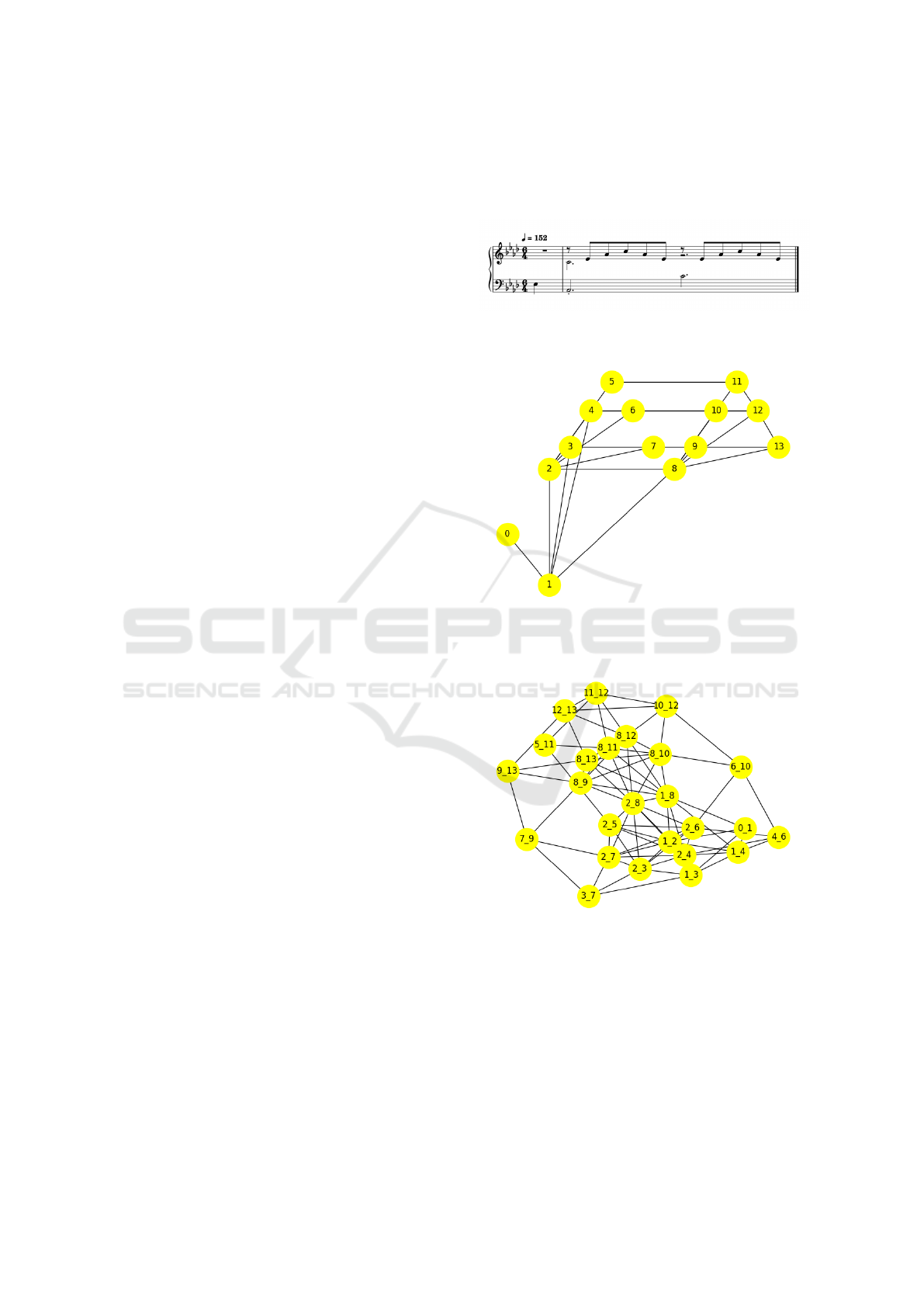
For illustration, Figures 1 and 2 show an extract

from Liszt’s Liebestraum and its corresponding

Szeto-Wong representation.

Step 3: Note Difference Graph Generation

From the Szeto-Wong graph, we generate our

novel “note difference graph” through the following

transformation process:

• Nodes: Each node represents an edge from the

original Szeto-Wong graph.

• Edges: Connect nodes in the note difference

graph that correspond to edges sharing a common

node in the original graph.

This transformation is visualized in Figure 3, where

node names correspond to the connected nodes from

Figure 2.

Figure 1: Extract of Liebestraum by Liszt.

Figure 2: Szeto and Wong Representation of Liebestraum

Extract.

Figure 3: Our Representation of Liebestraum Extract.

3.1.2 Node Encoding

Each node in our proposed graph is encoded with

three features:

1. Pitch Difference: Change in pitch values be-

tween connected notes.

2. Onset Difference: Difference in onset timing.

3. Temporal Gap: Time difference between the ﬁrst

KDIR 2025 - 17th International Conference on Knowledge Discovery and Information Retrieval

374

note’s end and the second note’s start.

Example Calculation: Consider nodes 0 and 1

from Figure 2:

• Node 0: Pitch = 51, Onset = 0, Duration = 1 beat.

• Node 1: Pitch = 44, Onset = 1, Duration = 3 beats.

The resulting node “0 1” in Figure 3 would have:

• Pitch Difference: −7 (44 − 51).

• Onset Difference: 1 (1 − 0).

• Temporal Gap: 0 (end of node 0 to start of node

1).

3.2 Graph Neural Network

Architecture

Graph Neural Networks operate differently from tra-

ditional neural networks as they are designed to han-

dle graph-structured data, which traditional networks

cannot process effectively. In a Graph Neural Net-

work, each layer applies operations to individual

graph components (nodes in our case) to produce

node embeddings. These operations incorporate in-

formation from neighbouring nodes at each layer, up-

dating node embeddings according to the layer’s spe-

ciﬁc function. This design enables Graph Neural

Networks to handle graphs of varying sizes, as lay-

ers operate at the component level rather than requir-

ing ﬁxed input dimensions like traditional neural net-

works.

Our classiﬁcation model employs a four-layer

graph neural network architecture designed speciﬁ-

cally for composer identiﬁcation (see Table 4). The

architecture follows established practices in music in-

formation retrieval while incorporating adaptations

for our novel graph representation.

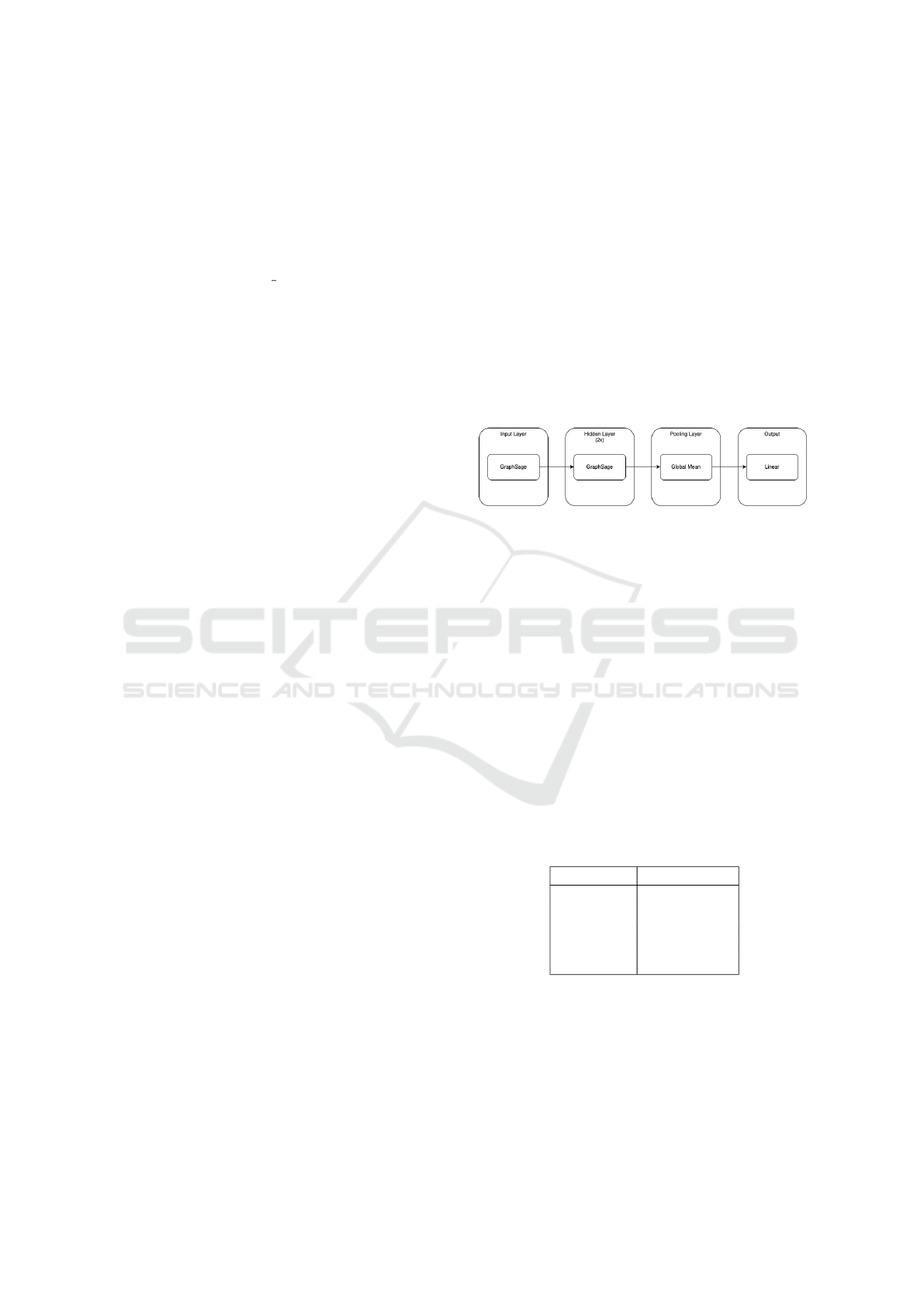
3.2.1 Network Structure

The model consists of four sequential components:

1. Input Layer: GraphSAGE convolutional layer

with 3 input dimensions corresponding to our

three node features (pitch difference, onset differ-

ence, and temporal gap)

2. Hidden Layers: Two additional GraphSAGE

convolutional layers, each with 75 hidden dimen-

sions following the conﬁguration used by Zhang

et al. (Zhang et al., 2023)

3. Pooling Layer: Global mean pooling layer that

aggregates node-level representations into a single

graph-level representation

4. Output Layer: Linear layer with 5 output dimen-

sions corresponding to the ﬁve composer classes

in our dataset, with each output representing the

probability of assignment to that composer

3.2.2 Architecture Details

The choice of GraphSAGE layers aligns with estab-

lished approaches in symbolic music classiﬁcation,

leveraging the inductive representation learning ca-

pabilities demonstrated by Hamilton et al. (Zhang

et al., 2023; Hamilton et al., 2017). The network em-

ploys ReLU activation functions throughout and ap-

plies dropout regularization (rate = 0.2) to all Graph-

SAGE layers to prevent overﬁtting.

Figure 4: Convolutional GNN Architecture.

4 DATASET

The dataset used in our research is a subset of the

GiantMIDI-Piano dataset provided by Kong et al.

(Kong et al., 2022). This dataset has transcribed live

recordings of classical piano music into MIDI repre-

sentations. Our subset contains all the works of Bach,

Chopin, Liszt, Schubert, and Scarlatti that the authors

recommend for training, testing, or validating. The

works of these composers are the ﬁve most numerous

in the dataset. This dataset was chosen as it is one of

the largest datasets available for MIDI ﬁles that also

contains composer labels. A summary of the number

of works can be seen in Table 1.

Table 1: Composers and their Works (Unbalannced).

Composer Work Count

Chopin 102

Liszt 197

Schubert 127

Scarlatti 274

Bach 147

Due to the imbalanced nature of the dataset, a sec-

ond balanced subset was constructed. This subset up-

sampled works by Chopin, Liszt, Schubert, and Bach

while undersampling works by Scarlatti. The new

dataset consists of 204 works for each composer. This

target was chosen to double the representation of the

smallest class (Chopin with 102 works) whilst main-

Composer Classiﬁcation Using a Note Difference Graph

375

taining a substantial sample size for evaluation. For

composers requiring upsampling, works were dupli-

cated to reach the target of 204. For overrepresented

composers, works exceeding 204 were randomly dis-

carded.

5 EXPERIMENTS

To evaluate the merits of our representation, we assess

how it performs in the task of composer classiﬁcation.

The results of this are then compared against the re-

sults obtained in the same task using the representa-

tion presented by Szeto and Wong (Szeto and Wong,

2006). Each representation is used to train a GNN.

These GNNs are then used to classify the composers

of unseen works. The experiments are performed on

the unbalanced and balanced datasets to ensure there

is not a bias towards overrepresented composers. It

should be noted that Szeto and Wong’s representation

was intended to be used for analysing post-tonal mu-

sic. Although the underlying goal of their paper is

different, their representation serves as a good point

of comparison for our own.

5.1 Description

For each experiment, the ordering of the dataset is

randomised. The dataset is then split so that 70%

of the data is used for training and 30% of the

data is used for testing. The GNN then iterates for

100 epochs. Observationally, no improvements were

made beyond this point. These experiments were

performed 10 times on each representation and each

dataset.

5.2 Statistical Signiﬁcance

To determine whether the improvements gained from

our proposed graph representation were statistically

signiﬁcant, we conducted additional experiments

comparing the representations. We created ﬁve pre-

determined randomisations of the unbalanced dataset

with the same 70%/30% training/test split as above.

Two GNNs are trained on the same randomisations

using their respective representations, and the out-

put from each model was compared using McNemar’s

test. This test is speciﬁcally designed to compare the

performance of two classiﬁers on the same dataset and

evaluates whether the observed differences in classi-

ﬁcation accuracy between the two approaches are sta-

tistically signiﬁcant or could be attributed to random

variation. The equation for this test can be seen in

Equation 1:

(|a − b| − 1)

a + b

(1)

• χ

: The calculated chi-square test statistic.

• b: Number of instances where Classiﬁer A is cor-

rect AND Classiﬁer B is incorrect.

• c: Number of instances where Classiﬁer A is in-

correct AND Classiﬁer B is correct.

6 RESULTS

The results of our experiments show that when our

representation was used to train the GNN it outper-

formed a GNN trained on data using the represen-

tation of Szeto and Wong. The GNN using our

representation achieved a classiﬁcation of 74% ac-

curacy using the unbalanced dataset and 74% ac-

curacy using the balanced dataset. These results

compare favourably with the representation of Szeto

and Wong, which achieved an average of 59% us-

ing the unbalanced dataset and a 53% on the bal-

anced dataset. In addition to the improved classiﬁ-

cation accuracy, the results of McNemar’s test pro-

duced a P-value of p < 0.001. This indicates that the

improvement in performance from our representation

is statistically signiﬁcant. The McNemar Test Table

from which the p value is derived can be seen in Ta-

ble 6. This improvement is exaggerated in the unbal-

anced dataset where the works of certain composers

are overrepresented and others are underrepresented.

6.1 Size Impact

While our approach has proven effective in increasing

composer classiﬁcation rates, it is worth highlighting

the increased space requirements of the representa-

tion. In the example shown in Figures 2 and 3, the

graph representation transforms from a graph with 14

nodes and 25 edges to a graph with 25 nodes and 83

edges. This increased size is further exaggerated for

larger pieces. A randomly selected Bach work was

examined to demonstrate the scaling effect. In this

work, the Szeto and Wong representation comprises

3,492 nodes and 15,353 edges. Transforming their

representation into our approach results in a graph

with 15,353 nodes and 152,784 edges.

This increased graph size results in longer training

times. To account for this computational discrepancy,

we performed an additional experiment in which a

GNN was trained on the Szeto and Wong approach

for an additional 600 epochs (700 total) to provide a

KDIR 2025 - 17th International Conference on Knowledge Discovery and Information Retrieval

376

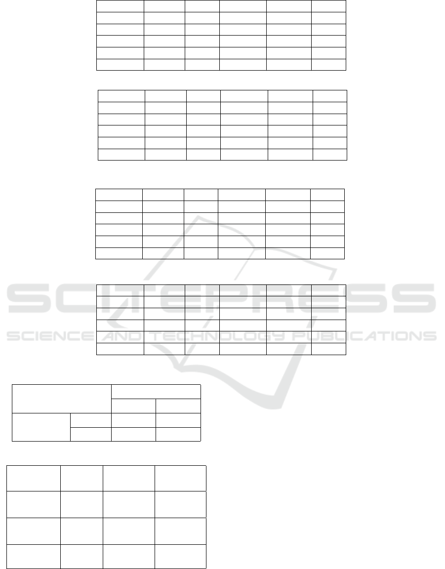
Table 2: Confusion Matrix of Our Representation.

Chopin Liszt Schubert Scarlatti Bach

Chopin 37.14 15.81 32.37 7.64 7.04

Liszt 5.9 78.16 13.24 1.18 1.52

Schubert 14.43 12.18 58.98 9.84 4.56

Scarlatti 1.09 0.11 2.81 86.39 9.6

Bach 1.75 2.21 1.75 10.26 84.03

Table 3: Confusion Matrix of Szeto and Wong Representation.

Chopin Liszt Schubert Scarlatti Bach

Chopin 2.08 63.14 15.55 13.8 5.43

Liszt 2.15 78.01 11.3 6.15 2.38

Schubert 1.03 44.84 28.29 15.42 10.42

Scarlatti 0.12 4.3 1.04 90.34 4.2

Bach 0.65 11.1 5.3 49.33 33.61

Table 4: Confusion Matrix of Our Representation on a Balanced Dataset.

Chopin Liszt Schubert Scarlatti Bach

Chopin 62.35 13.73 20.74 1.09 2.09

Liszt 11.55 73.69 12.64 0.82 1.3

Schubert 17.44 7.92 71.28 2.89 0.46

Scarlatti 2.02 0.17 3.96 86.81 7.04

Bach 4.53 1.1 3.85 15.88 74.65

Table 5: Confusion Matrix of Szeto and Wongs Representation on a Balanced Dataset.

Chopin Liszt Schubert Scarlatti Bach

Chopin 26.22 46.96 19.67 6.84 0.3

Liszt 16.73 66.52 12.03 4.72 0.0

Schubert 21.11 27.66 36.89 13.38 0.96

Scarlatti 3.53 2.65 6.52 87.29 0.0

Bach 9.47 9.25 21.94 23.86 35.48

Table 6: McNemar’s Test Table.

Note Diff. Graph Model

Correct Incorrect

Szeto & Wong

Graph Model

Correct 505 179

Incorrect 435 156

Table 7: Model Performance Comparison.

Approach Epochs

Time

(Seconds)

Accuracy

(%)

Szeto

& Wong

100 9763.41 0.57%

Szeto

& Wong

700 65034.82 0.65%

Conlin &

O’Riordan

100 59948.63 0.75%

more comparable training duration. As shown in Ta-

ble 7, even with extended training time, the classiﬁ-

cation accuracy using the Szeto and Wong represen-

tation remains lower than the accuracy achieved with

our representation.

7 OBSERVATIONS

Looking past the overall classiﬁcation score we can

observe that both the GNNs had greater difﬁculty dif-

ferentiating between the works of Chopin, Liszt and

Schuber. This is similarly observed between Scarlatti

and Bach. This observation can be seen in Tables 2 -

5. The rows in these tables are the ground truth and

the columns are the predictions.

Although Szeto and Wong’s representation per-

formed better in the unbalanced dataset (Table 3)

compared to the balanced one (Table 5), this appears

to be a result of an over-representation of Scarlatti and

Liszt and an under-representation of Chopin. We can

observe in Table 3 that the representation was only

able to identify Scarlatti and Liszt correctly more than

Composer Classiﬁcation Using a Note Difference Graph

377

other composers. The rest were classiﬁed as another

composer rather than the correct composer. This re-

sulted in producing a higher average than with the

balanced dataset despite producing better results for

the other composers in the balanced dataset as seen

in Table 5. This shows that Szeto and Wong’s rep-

resentation was more prone to bias with imbalanced

datasets.

In contrast, our approach was much less prone to

bias, correctly identifying all the composers as them-

selves rather than another composer. This is seen

along the diagonal in Table 2 and Table 4 where the

diagonal should contain the highest value of that row.

8 DISCUSSION

A look into the time periods in which the composers

were most active might offer some insight into the

misclassiﬁcation reported by the GNN. Both Chopin

and Liszt were most active in the Romantic era, Schu-

bert was active the late classical to early romantic era,

and Scarlatti and Bach were active in the Baroque

era. The era in which the composers were most ac-

tive tends to correlate to the misclassiﬁcations of the

GNN. That is to say, Chopin, Liszt and Schubert were

more likely to get confused with one another due to

their work being in the romantic era. Similarly for

Scarlatti and Bach in the Baroque era. This might

suggest that the GNN is identifying compositional

choices common to those eras, but further research

would be required to conﬁrm this.

9 CONCLUSION

We have demonstrated a graph representation for

symbolic music that when used with a GNN outper-

forms other representations at the task of composer

classiﬁcation. We believe that our representations fo-

cus on the relationships between notes provide the

GNN with a more intuitive understanding of what is

important within a composition.

An issue with our representation can be seen in the

way edges are formed for the initial graph representa-

tion. With sequential edges connecting a note to the

next nearest note, there is a bias towards the X-axis.

This is because the x and y axes are weighted equally

in terms of distance. A note that is one beat away at

the same pitch is seen to be nearer than a note that is

a quarter beat away that is an octave higher as seen

in Figure 2. Further work is required to address this

edge connection issue.

REFERENCES

Collins, T., Arzt, A., Flossmann, S., and Widmer, G. (2013).

Siarct-cfp: Improving precision and the discovery of

inexact musical patterns in point-set representations.

In ISMIR, pages 549–554.

Collins, T. and Meredith, D. (2013). Maximal transla-

tional equivalence classes of musical patterns in point-

set representations. In Mathematics and Computation

in Music: 4th International Conference, MCM 2013,

Montreal, QC, Canada, June 12-14, 2013. Proceed-

ings 4, pages 88–99. Springer.

Collins, T., Thurlow, J., Laney, R., Willis, A., and

Garthwaite, P. (2010). A comparative evaluation of

algorithms for discovering translational patterns in

baroque keyboard works. Proceedings of the 11th

International Society for Music Information Retrieval

Conference, ISMIR 2010.

Conklin, D. and Witten, I. H. (1995). Multiple viewpoint

systems for music prediction. Journal of New Music

Research, 24(1):51–73.

Corr

ea, D. C. and Rodrigues, F. A. (2016). A survey on

symbolic data-based music genre classiﬁcation. Ex-

pert Systems with Applications, 60:190–210.

Forth, J. and Wiggins, G. A. (2009). An approach for identi-

fying salient repetition in multidimensional represen-

tations of polyphonic music. London Algorithmics

2008.

Hamilton, W. L., Ying, R., and Leskovec, J. (2017). Induc-

tive representation learning on large graphs. CoRR,

abs/1706.02216.

Jeong, D., Kwon, T., Kim, Y., and Nam, J. (2019). Graph

neural network for music score data and modeling ex-

pressive piano performance. In International confer-

ence on machine learning, pages 3060–3070. PMLR.

Karystinaios, E. and Widmer, G. (2022). Cadence detec-

tion in symbolic classical music using graph neural

networks. arXiv preprint arXiv:2208.14819.

Karystinaios, E. and Widmer, G. (2023). Roman numeral

analysis with graph neural networks: Onset-wise pre-

dictions from note-wise features. arXiv preprint

arXiv:2307.03544.

Kong, Q., Li, B., Chen, J., and Wang, Y. (2022). Giantmidi-

piano: A large-scale midi dataset for classical piano

music.

Lemstr

om, K. and Pienim

aki, A. (2007). On comparing edit

distance and geometric frameworks in content-based

retrieval of symbolically encoded polyphonic music.

Musicae Scientiae, 11(1 suppl):135–152.

Li, X., Ji, G., and Bilmes, J. A. (2006). A factored language

model of quantized pitch and duration. In ICMC. Cite-

seer.

Meredith, D. (2013). Cosiatec and siateccompress: Pattern

discovery by geometric compression. In International

society for music information retrieval conference. In-

ternational Society for Music Information Retrieval.

Meredith, D. (2016). Using siateccompress to discover re-

peated themes and sections in polyphonic music. In

Music Information Retrieval Evaluation Exchange.

KDIR 2025 - 17th International Conference on Knowledge Discovery and Information Retrieval

378

Meredith, D., Wiggins, G., Lemstr

om, K., and Music, P.

(2002). A geometric approach to repetition discovery

and pattern matching in polyphonic music. Computer

Science Colloquium.

Mokbel, B., Hasenfuss, A., and Hammer, B. (2009). Graph-

based representation of symbolic musical data. In

Graph-Based Representations in Pattern Recognition:

7th IAPR-TC-15 International Workshop, GbRPR

2009, Venice, Italy, May 26-28, 2009. Proceedings 7,

pages 42–51. Springer.

Pearce, M. and Wiggins, G. (2004). Improved methods for

statistical modelling of monophonic music. Journal of

New Music Research, 33.

Pearce, M. T. (2018). Statistical learning and probabilistic

prediction in music cognition: mechanisms of stylistic

enculturation. Annals of the New York Academy of

Sciences, 1423(1):378–395.

Pinto, A. and Tagliolato, P. (2008). A generalized graph-

spectral approach to melodic modeling and retrieval.

In Proceedings of the 1st ACM international confer-

ence on Multimedia information retrieval, pages 89–

96.

Schedl, M., G

omez, E., Urbano, J., et al. (2014). Music

information retrieval: Recent developments and ap-

plications. Foundations and Trends® in Information

Retrieval, 8(2-3):127–261.

Sturm, B. L. (2014). The state of the art ten years after a

state of the art: Future research in music information

retrieval. Journal of new music research, 43(2):147–

172.

Szeto, W. M. and Wong, M. H. (2006). A graph-theoretical

approach for pattern matching in post-tonal music

analysis. Journal of New Music Research, 35.

Ukkonen, E., Lemstr

om, K., and M

akinen, V. (2003a). Ge-

ometric algorithms for transposition invariant content-

based music retrieval. ISMIR.

Ukkonen, E., Lemstr

om, K., and M

akinen, V. (2003b).

Sweepline the music. Computer Science in Perspec-

tive: Essays Dedicated to Thomas Ottmann, pages

330–342.

Wiggins, G. A., Lemstr

om, K., and Meredith, D. (2002).

Sia (m) ese: An algorithm for transposition invariant,

polyphonic content-based music retrieval. In ISMIR.

Zhang, H., Karystinaios, E., Dixon, S., Widmer, G., and

Cancino-Chac

on, C. E. (2023). Symbolic music repre-

sentations for classiﬁcation tasks: A systematic eval-

uation. arXiv preprint arXiv:2309.02567.

Zhao, T., Zhang, X., and Wang, S. (2021). Graphsmote:

Imbalanced node classiﬁcation on graphs with graph

neural networks. CoRR, abs/2103.08826.

Zhou, Y., Zheng, H., Huang, X., Hao, S., Li, D., and Zhao,

J. (2022). Graph neural networks: Taxonomy, ad-

vances, and trends. ACM Transactions on Intelligent

Systems and Technology (TIST), 13(1):1–54.

Composer Classiﬁcation Using a Note Difference Graph

379