
Enhanced Face Reconstruction and Recognition System with
Audio-Visual Fusion
Prathika Muthu, Damodharan Asaithambi Ramani and Jenifer Arputham
Artificial Intelligence and Data Science, St.Joseph’s Institute of Technology,Chennai,Tamilnadu, India
Keywords: Audio-Visual Fusion, Face Reconstruction, Face Recognition, Local Binary Pattern (LBP), Radon Transform,
Autoencoder, Convolutional Neural Network (CNN)
Abstract: Deep Learning-Based Audio-Visual Fusion Approach for Enhanced Face Reconstruction and Recognition
System: A New Paradigm for Improving Accuracy of Face Reconstruction and Recognition. The challenging
factors in this area, namely illumination, pose, and expression, have been addressed by Local Binary Pattern
over Radon Transform audio feature extraction that are fused with visual data. The features are encoded with
an autoencoder while the CNN-based decoder reconstructs facial images of high quality from noisy or
incomplete data. This innovative system will improve the accuracy of recognition in any scenario, making it
valuable for forensic analysis, security, and adaptive user interfaces. Audio-visual fusion can be used to
perform holistic facial analysis, which is far beyond the traditional visual-only approach. Advanced neural
networks provide much better performance than existing approaches. Future extensions could include thermal
imaging, depth data, or real-time processing for dynamic environments. This system, based on deep learning
techniques, marks an important step in facial recognition technology with great potential applications across
various domains that require reliable and precise facial identification.
1 INTRODUCTION
Using audio descriptions and visual data to produce
better face reconstruction and identification accuracy,
the “Enhanced Face Reconstruction and Recognition
System Using Deep Learning with Audio-Visual
Fusion” is a paradigm leap in facial recognition
technology. Among the many serious drawbacks of
traditional facial recognition systems is their inability
to process visual data that is unclear, loud, or missing.
Their effectiveness is hampered by these limitations
in situations with different lighting conditions,
postures, and facial expressions—all of which are
crucial for real-world applications like security and
forensic investigation. To address these challenges,
the proposed system integrates audio and visual
inputs for a holistic analysis of facial features.
Essential contextual information is provided by audio
data, which is frequently underused in facial
recognition. Because of its resilience in identifying
directional patterns and textures in sound waves, the
Local Binary Pattern over Radon Transform (LBRP)
is used to extract significant features from audio
descriptions. To improve the portrayal of face
characteristics, these traits are combined with visual
information. A sophisticated deep earning framework
is used in the system architecture. High dimensional
face traits are encoded by an autoencoder technique,
which guarantees effective compression while
maintaining important data. From the encoded data, a
CNN-based decoder that uses transposed convolution
reconstructs high-fidelity face pictures. Transposed
convolution was chosen in particular because it can
efficiently up sample features while preserving
spatial consistency and guaranteeing high-quality
reconstruction even when inputs are noisy or
insufficient. By combining audio-visual data, the
system is in a unique position to perform better than
conventional techniques and adjust to difficult
situations such different lighting, postures, and facial
expressions. Among the contributions of the system
are utilizing audio-visual fusion to overcome the
shortcomings of conventional technologies.
Presenting LBRP, an efficient method for extracting
audio features that enhance visual data .utilizing a
strong architecture that combines CNNs and
autoencoders to achieve accurate reconstruction.
Future improvements can include using bigger and
more varied datasets, enabling real-time processing in
dynamic contexts, and integrating speech patterns
Muthu, P., Asaithambi Ramani, D. and Arputham, J.
Enhanced Face Reconstruction and Recognition System with Audio- Visual Fusion.
DOI: 10.5220/0013734400004664
Paper published under CC license (CC BY-NC-ND 4.0)
In Proceedings of the 3rd International Conference on Futuristic Technology (INCOFT 2025) - Volume 3, pages 887-894
ISBN: 978-989-758-763-4
Proceedings Copyright © 2025 by SCITEPRESS – Science and Technology Publications, Lda.
887
and emotional tones with auditory data. These
developments will improve the system’s functionality
even more and broaden its use in fields that demand
accurate and dependable facial recognition.
2 RELATED WORKS
A diffeomorphic volume-to-slice registration
approach with a deep generative prior to address
motion artifacts in prenatal MRI, achieving robust
volumetric reconstruction. Validated on 72 fetal
datasets (20–36 weeks gestation), it outperformed
state-of-the-art techniques with a mean absolute error
of 0.618 weeks and R² = 0.958 for gestational age
prediction, with accuracy further enhanced by
combining brain and trunk data. (Grande, et al. ,
2023)Benefits include superior image quality and
comprehensive fetal analysis, while limitations
involve high computational complexity and the need
for broader validation across diverse imaging
conditions. Using min-max concave (MC) penalties
for unbiased sparse constraints and total variation
(TV) for uniform intensity, it suggests a nonconvex
regularization technique for Magnetic Particle
Imaging (MPI). The method improves reconstruction
accuracy by employing an alternate direction method
of multipliers (ADMM) and a two step parameter
selection process. (Zhu, et al. , 2024)
It decreased intensity error from 28 percent to 8
percent when tested on OpenMPI, simulations, and
hand-help scanner data. While there are benefits like
better picture quality and accurate quantitative
characteristics, there are drawbacks including
computational complexity and the requirement for
more extensive real-world validation.By integrating
image priors, kernelized expectation maximization
(KEM) aids in the difficult task of reconstructing low-
count PET data. In order to improve reconstruction,
this work presents implicit regularization using a
deep coefficient prior, which is represented by a
convolutional neural network. To ensure monotonic
likelihood improvement, the suggested neural KEM
method alternates between a deep-learning phase for
updating kernel coefficients and a KEM step for
image updates. It performed better than conventional
KEM and deep image prior techniques, as confirmed
by simulations and patient data. (Gong, Badawi, et al.
, 2023)
Improved reconstruction accuracy and effective
optimization are benefits; nevertheless,
computational complexity and the requirement for
further clinical validation are drawbacks. Positronium
lifetime (PLI), which is impacted by tissue
microenvironments, is captured by Positron Emission
Tomography (PET) imaging, providing information
on the course of illness. A statistical image
reconstruction technique for high-resolution PLI is
presented in this work, which includes a correction
for random triple coincidence occurrences that is
essential for real-world uses. The technique may
provide life time pictures with high accuracy, low
variation, and resolution similar to PET activity
images utilizing the existing time of flight resolution,
as shown by simulations and experimental
investigations. (Guan, et al. , 2024).
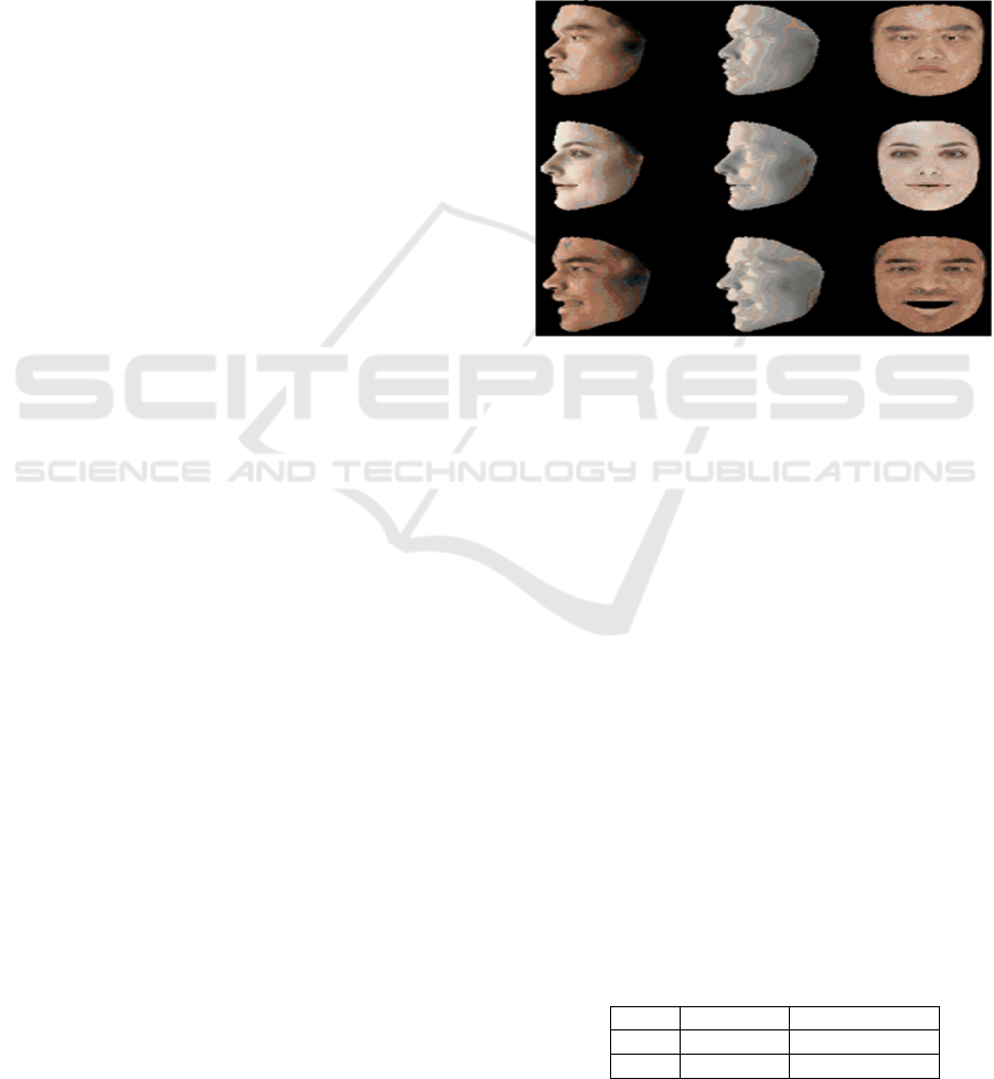
Figure 1: Face Recognition
3 METHODOLOGY
3.1 Dataset
The ”Labeled Faces in the Wild” (LFW) dataset is a
widely used benchmark for studying unconstrained
face recognition.
It organizes images into folders labeled by
individual names, with each folder containing
samples of that person. Captured in real-world
conditions, the dataset presents challenges such as
varying lighting, poses, and occlusions. Aligned
facial land marks, including the eyes, nose, and
mouth, ensure uniformity enhancing the performance
of deep learning models. LFW is particularly valuable
for tasks like face verification and person
reidentification as many individuals have multiple
images.it includes diverse facial expressions and
angles, making it ideal for robust model training and
evaluation.
Table 1:Dataset Statistics
S.No Name No.of Images
1 LFW 13233
2 CELEBA 202599
INCOFT 2025 - International Conference on Futuristic Technology
888
3.2 DataCollection:
Images of faces are collected from datasets that
include images of various poses, lighting conditions,
expressions, and even occlusions: CelebA, LFW,
CASIA-WebFace. Audio descriptions include sound
and pitch; timestamps are provided and aligned to
corresponding facial features in the collection so that
every audio feature would correspond to a
corresponding video frame even in cases of dynamic
scenarios. For example, mapping audio descriptors
like pitch and energy to the properties of video frames
adds up to the accuracy. Data validation comes in to
ensure that the data is well-organized and of good
quality, ensuring meaningful results from the
analysis.It ensures proper integration of audio and
visual information.
3.3 Data Preprocessing:Audio-Video:
Resizing: Resizing will ensure all images fed into a
machine learning model have an equalized pixel
resolution. This is quite crucial in providing
consistency on all fronts. Preprocessing through
resizing yields images with identical
dimensionalities, which is helpful for the model.
However, resizing can sometimes alter the aspect
ratio, and this is retained to minimize distortion
further. Some common ones are the nearest
neighbour, bilinear, and bicubic. Resizing
standardizes the input but data loss will also be at a
greater risk, especially if the images get compressed.
Normalization: The homogeneity of normalizing
pixel values within a standard range of 0 to 1 or -1 to
1 improves model performance during pre-
processing. This gives a fast convergence, avoids
instability at any possible point, and provides equal
contribution of all pixels.
Data Augmentation: Rotating images by, for
instance ±15° or ±30° forces the model to detect
objects without regard to their angle. The horizontal
or vertical flip allows the model to handle elements
reflected over one axis. Shifting image along both
axes x and y improves the model’s ability to identify
objects at various positions, thus position-invariant.
Noise Reduction:The process of audio
preprocessing ensures that noise removal takes place,
thus ensuring that there is clear feature extraction.
Amongst some of the techniques which have been
used to that noise removal takes place, thus ensuring
that there clear feature extraction. Amongst some of
the techniques which have been used to that noise
removal takes place, thus ensuring that there clear
feature extraction have been used to reduce unwanted
frequencies are: spectral subtraction, band-pass
filtering, and high/low-pass filtering. wavelet
denoising, which clean the audio signal and post
Denoising procedures include Wiener filtering and
processing smoothing, which helps prevent artifacts.
To make sure that every audio feature matches the
corresponding visual frame, audio and visual inputs
are timestamped and along throughout data
collection. Pitch and energy are examples of audio
descriptors that are translated to the temporal
properties of the video frames in dynamic situations.
Feature Extraction using LBRP: The Local
Binary Radon Pattern technique is a process where
audio features are extracted through local textures
and directional patterns. Similar to this, it compares
short frames of audio signals that capture how the
energy of the sound changes along time and applies
the Radon transform to determine the shift in
directions. Then, it assists in correlating the auditory
cues to visual data ; this performs better
reconstruction of faces from audio descriptions.
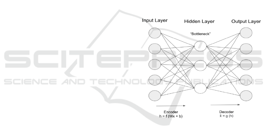
Figure 2: Component Diagram
3.4 Decoding of Encoder
Input Layer: The input to the encoder is a high-
dimensional data vector, such as a facial image
represented by pixel values.Let the input data be
denoted as:
x ∈𝑅
(1)
where n is the dimensionality of the input data
(e.g., the number of pixels in an image).
Fully Connected/Convolutional Layers: In an
encoder that has a deep learning approach, the input
passes through several layers, all of which are fully
connected or convolutional. These layers apply
transformations to learn feature representations. Let’s
Enhanced Face Reconstruction and Recognition System with Audio- Visual Fusion
889
take the fully connected layer, where the
transformation is given by:
h = f (W x + b) (2)
where:
• h is the hidden layer (compressed feature
representation),
• W is the weight matrix of the layer,
• b is the bias vector,
• f (·) is an activation function such as ReLU
(Rectified Linear Unit).
For a convolutional layer, the transformation
involves convolution operations:
ℎ
(
)
=𝑓
∑∑
𝑊
()
𝑥
.
+𝑏
()
(3)
where:
• 𝑊
()
is the convolution kernel (filter) of size
M × N ,
• 𝑥
,
is the local patch of the input
centered at (i, j),
• f (·) is the activation function (e.g., ReLU).
Pooling/Downsampling Layers: Pooling layers
are used to reduce the dimensionality and focus on the
most important features. A common type of pooling
is max pooling, where the transformation is given by:
ℎ
=maxℎ
,
(4)
This operation reduces the spatial dimensions by
taking the maximum value from a patch of the feature
map, which decreases the resolution but preserves
significant features. Bottleneck Layer: By
condensing high-dimensional inputs into a single
latent space, the autoencoder’s bottleneck layer
efficiently captures the combined representation of
audio and visual characteristics. Important aspects of
both senses are combined, maintaining connections
like the way some auditor signals correspond with
visual patterns. Even with noisy or incomplete data,
this latent representation guarantees reliable encoding
of crucial, complementary information, allowing for
precise reconstruction. It can be mathematically
represented as:
𝑧=𝑓(𝑊
ℎ+𝑏
) (5)
where:
• z is the low-dimensional embedding or
latent space representation of the input,
• 𝑊
is the weight matrix of the bottleneck
layer,
• 𝑏
is the bias vector of the bottleneck
layer,
• f (·) is an activation function (e.g.,
ReLU).
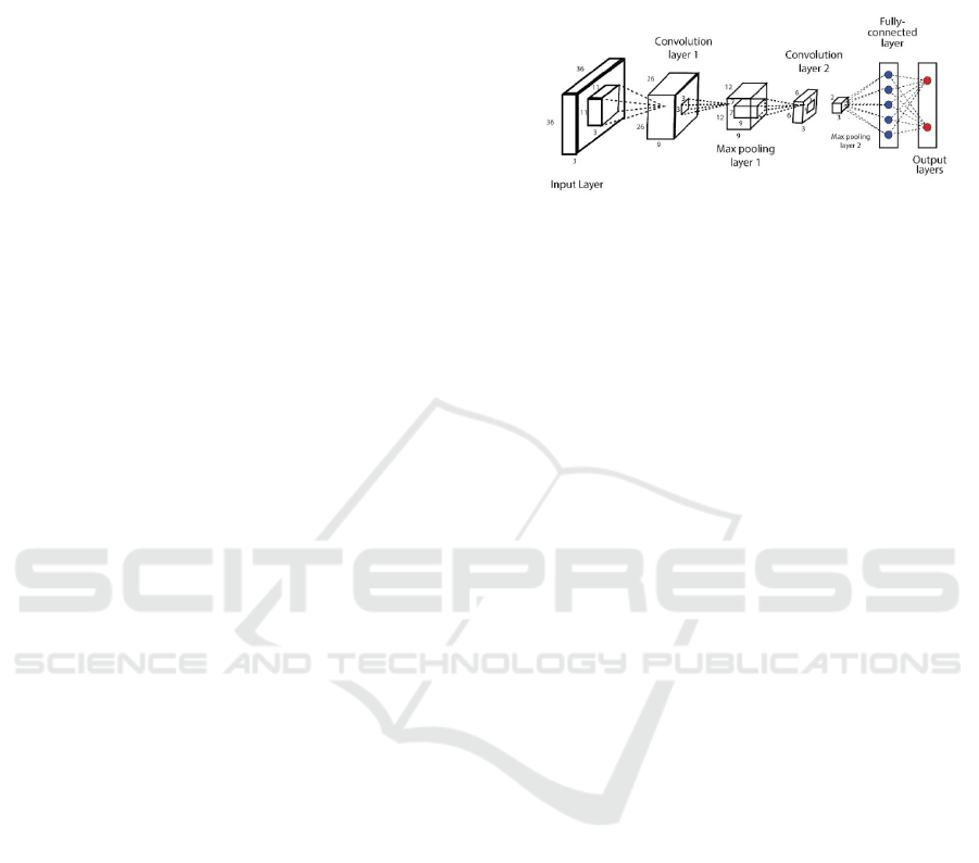
Figure 3: System Architecture
3.5 Decoding of CNN
In a Convolutional Neural Network (CNN)- based
decoder architecture, the decoder reconstructs an
image from a com pressed representation (often
produced by an encoder or some fused features).
Input from Encoder (Compressed Features):
The decoder takes the compressed feature map from
the encoder. This compressed data encapsulates
important high-level features of the original image.
Transposed Convolution Layers
(Deconvolution):The core part of a CNN decoder is
the transposed convolution layers. These layers are
used to upsample the compressed feature map to a
higher resolution, typically back to the size of the
original image. The output dimensions of a
transposed convolution layer can be computed using
the following formula:
𝐻
=
(
𝐻
−1
)
×𝑆+𝐾−2𝑃 (6)
𝑊
=
(
𝑊
−1
)
×𝑆+𝐾−2𝑃 (7)
where:
• 𝐻
and 𝑊
are the height and width
of the output feature map,
• 𝐻
and 𝑊
are the height and width of
the input feature map,
• S is the stride,
• K is the kernel size,
• P is the padding applied.
The transposed convolution layers gradually
increase the resolution, reconstructing the spatial
structure of the image.
ReLU Activation Function: After each
transposed convolution layer, the ReLU (Rectified
Linear Unit) activation function is typically applied
to introduce non-linearity, helping the decoder learn
complex patterns The function is defined as:
INCOFT 2025 - International Conference on Futuristic Technology
890

f(x)=max(0,x) (8)
where x is the input. This ensures that only
positive values are passed on, effectively handling the
non-linearity of the data.
Final Convolution Layer: The final layer of the
CNN decoder is typically a convolution layer with a
sigmoid activation function, which maps the feature
maps to the correct number of channels (for example,
1 for grayscale images or 3 for RGB images).
𝜎
(
𝑥
)
=
(9)
This function normalizes the output pixel values
between 0
and 1.
Loss Calculation (Reconstruction Error): The
reconstructed image is compared to the original
image using a loss function like Mean Squared Error
(MSE).
𝑀𝑆𝐸 =
∑
(𝑦
𝑦
)
(10)
where:
• 𝑦
is the true pixel value,
• 𝑦
is the predicted pixel value.
The MSE measures the difference between the
original and
the reconstructed image.
3.6 Face Recognition
Feature Embedding: In CNN-based face
recognition, after the encoder extracts features from
the input image, the features are mapped into a fixed-
length embedding vector. This embedding represents
the unique characteristics of a face, enabling com
parison across different images.We define the output
of the fully connected (FC) layer as:
e = FC (f (x)) = W · f (x) + b (11)
where f (x) represents the features extracted by the
CNN encoder from the input image x, W is the weight
matrix, and b is the bias vector.
Similarity Measurement: To determine whether
two faces are similar (or belong to the same person),
we compute the similarity between their embedding
vectors. Two commonly used similarity metrics are:
a) Cosine Similarity: The cosine similarity
between two embedding vectors e1 and e2 is given
by:
𝑆
(
𝑒
,𝑒
)
=
.
‖
‖‖
‖
(12)
where e1 and e2 are two embedding vectors and
∥e∥ represents the magnitude (L2 norm) of vector e.
b) Euclidean Distance: The Euclidean distance
between two embedding vectors e1 and e2 is given
by:
𝑑
(
𝑒
,𝑒
)
=
‖
𝑒
−𝑒
‖
=
∑
(
𝑒
−𝑒
)
(13)
where e1i and e2i are the components of the
embedding vectors e1 and e2, respectively.
The smaller the Euclidean distance, or the closer
the cosine similarity is to 1, the more similar the two
embeddings, and thus, the more likely they represent
the same individual.
3.7 Classifiation
Once the similarity score (cosine similarity or
Euclidean distance) is obtained, the next step is to
classify the identity of the individual.
Softmax Function: When you have multiple
classes (identities), you can use a softmax activation
to convert similarity scores into probabilities. The
identity with the highest probability is selected as the
predicted class. The softmax function is defined as:
𝑃
=
∑
(14)
where zi is the similarity score for class i, and
∑
𝑒
is the sum of the exponentials of similarity
scores over all classes.
The identity corresponding to the highest 𝑃
is
chosen as the predicted class.
Sigmoid Function (for Binary Classification):
If the goal is to classify whether the face matches a
specific identity (binary classification), the sigmoid
activation function can be used:
𝑃
=
(15)
where zi is the similarity score. The output will be
a value between 0 and 1, representing the probability
that the face matches the given identity. A value
closer to 1 indicates a match, while a value closer to
0 indicates no match.
Enhanced Face Reconstruction and Recognition System with Audio- Visual Fusion
891

3.8 Training process
To teach the Autoencoder and CNN models, we feed
them data and use specific metrics to see how well
they’re learning.
For the Autoencoder, we measure how closely the
output matches the input using a ”Mean Squared
Error” measure. For the CNN, which focuses on
recognizing patterns, we use a Cross-Entropy”
measure to assess how well it’s making predictions.
3.9 Fine Tuning Process
We experiment with different settings, such as how
fast the model learns (learning rate), how many data
points we process at a time (batch size), and the
structure of the model itself. This tweaking helps us
improve the model’s performance.
4 PERFORMANCE METRICS
Accordingly, various performance indicators are used
to evaluate the effectiveness of the suggested deep
learning system for malignant cell detection.
Accuracy: Accuracy represents how frequently
the model correctly classifies instances as cancerous
or not. It is calculated based on true positives (TP),
true negatives (TN),
false positives (FP), and false negatives (FN).
The formula for accuracy is given by:
𝐴𝑐𝑐𝑢𝑟𝑎𝑐𝑦 =
(16)
Precision: Precision indicates how many of the
instances that the model revealed as positive, or
cancerous, are actually correct. It measures the
accuracy of the model in predicting positive cases.
The formula for precision is:
𝑃𝑟𝑒𝑐𝑖𝑠𝑖𝑜𝑛 =
(17)
Recall(Sensitivity): Recall, also known as
sensitivity, quantifies how well the model identifies
actual positive cases. It displays the ratio of true
positives to the total number of actual positives
(TP+FN):
𝑅𝑒𝑐𝑎𝑙𝑙 =
(18)
F-1 score: The F1-Score is the harmonic mean of
recall and precision. It is particularly useful in cases
where there is a class imbalance. The formula for F1-
Score is:
𝐹1 − 𝑆𝑐𝑜𝑟𝑒 = 2 ×
×
×
(19)
ROC-AUC: The Receiver Operating
Characteristic curve (ROC) plots the true positive rate
(recall) against the false positive rate at different
threshold values. The Area Under the Curve (AUC)
is a summary measure of how well the model
distinguishes between classes. A higher AUC value
indicates better performance.
5 RESULT
Integration of both auditory and visual data enables
deep learning techniques to advance methods of face
reconstruction along with detection. The system will
require specific hardware that involves features of a
GPU that has CUDA support,like the NVIDIA RTX
series, 16GB RAM to process data, high-speed SSD
for holding big datasets, and a multicore CPU such as
Intel i7 or AMD Ryzen series to carry out
preprocessing and inference tasks.
It consists of three major datasets: Labeled Faces
in the Wild (LFW), with 13,233 images,and CelebA
with 202,599 images, and CASIA-WebFace, all of
which are used as training data sets to achieve
diversity and robustness in the model.
It should have Python 3.x as its primary
programming language, along with the installation of
TensorFlow or PyTorch to create a deep learning
model and train it; OpenCV to pre-process the image;
Librosa to extract audio features; and NumPy, Pandas
to handle the data.It uses Local Binary Pattern over
Radon Transform or LBRP for extracting audio
features and combines this with a visual. The system,
besides that, overcomes problems due to pose
variations, variability in lighting, and inadequate or
noisy input data as well.It applies an autoencoder for
the efficient encoding of features and a CNN-based
decoder for reconstructing images with good
quality.The system is compatible with Linux (for
example, Ubuntu 20.04) or Windows 10/11.
Tools such as Jupyter Notebook or Google Colab
are used for development and experimentation.
Version control is ensured using Git, and
environment replication is made easier using
Docker.This leads to a significant improvement in the
accuracies of facial reconstruction and recognition
estimated to be between 90%and 95%, effectively
INCOFT 2025 - International Conference on Futuristic Technology
892
making it suitable for deployment in forensic
analysis, security, and real-time adaptive interfaces.
Future development of the system may include
enhancements in real-time processing of images,
increased datasets, and the inclusion of advanced
auditory cues like speech patterns, emotional tones,
etc, to enhance the accuracy as well as generalization.
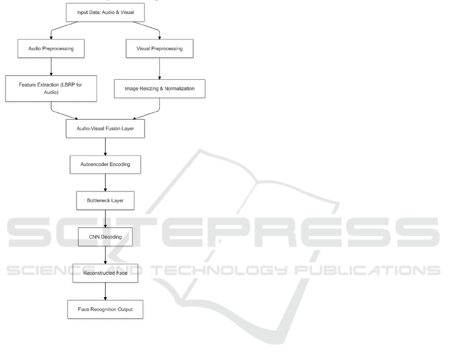
Figure 4 : Activity Diagraam
6 CONCLUSION
The proposed audio-visual fusion system greatly
enhance face reconstrction and recognition as it is
capable of mitigating the limitations of traditional
approaches: noisiness, incompleteness, or
inconsistency in data. However, there are several
limitations to its current applications such as a
dependence on high computational resources,
possible bias because of a lack of diversity of data
sets, and non-real-time applicability in processing.
Future research should be directed toward integrating
larger and diverse datasets, incorporating higher level
auditory cues such as tones of emotion and speech,
and optimization of architecture with respect to real-
time systems. Another direction can also be multi-
modal data fusion and edge computing; however,
emerging technologies should find their ways to
further optimize systems in terms of efficiency,
accuracy, and adaptability across real-world
scenarios.
REFERENCES
Cordero-Grande, L., et al. (2023). Fetal MRI by robust deep
generative prior reconstruction and diffeomorphic
registration. IEEE Transactions on Medical Imaging,
42(3), 810-822.
Zhu, T., et al. (2024). Accurate concentration recovery for
quantitative magnetic particle imaging reconstruction
via nonconvex regularization. IEEE Transactions on
Medical Imaging, 43(8), 2949-2959.
Li, S., Gong, K., Badawi, R. D., Kim, E. J., Qi, J., & Wang,
G. (2023). Neural KEM: A kernel method with deep
coefficient prior for PET image reconstruction. IEEE
Transactions on Medical Imaging, 42(3), 785-796.
Guan, Y., et al. (2024). Learning-assisted fast
determination of regularization parameter in
constrained image reconstruction. IEEE Transactions
on Biomedical Engineering, 71(7), 2253-2264.
Huang, B., et al. (2024). SPLIT: Statistical positronium
lifetime image reconstruction via time-thresholding.
IEEE Transactions on Medical Imaging, 43(6), 2148-
2158.
Fan, H., et al. (2024). High accurate and efficient 3D
network for image reconstruction of diffractive-based
computational spectral imaging. IEEE Access, 12,
120720-120728.
Salomon, A., Goedicke, A., Schweizer, B., Aach, T., &
Schulz, V. (2011). Simultaneous reconstruction of
activity and attenuation for PET/MR. IEEE
Transactions on Medical Imaging, 30(3), 804-813.
Zhou, S., Deng, X., Li, C., Liu, Y., & Jiang, H. (2023).
Recognition-oriented image compressive sensing with
deep learning. IEEE Transactions on Multimedia, 25,
2022-2032.
Mohana, M., & Subashini, P. (2023). Emotion recognition
using deep stacked autoencoder with softmax classifier.
2023 Third International Conference on Artificial
Intelligence and Smart Energy (ICAIS), 864-872
Abdolahnejad, M., & Liu, P. X. (2022). A deep autoencoder
with novel adaptive resolution reconstruction loss for
disentanglement of concepts in face images. IEEE
Transactions on Instrumentation and Measurement, 71,
1-13
Bragin, A. K., & Ivanov, S. A. (2021). Reconstruction of
the face image from speech recording: A neural
networks approach. 2021 International Conference on
Quality Management, Transport and Information
Security, Information Technologies (ITQMIS), 491-
494.
Gao, Y., Gao, L., & Li, X. (2021). A generative adversarial
network based deep learning method for low-quality
Enhanced Face Reconstruction and Recognition System with Audio- Visual Fusion
893

defect image reconstruction and recognition. IEEE
Transactions on Industrial Informatics, 17(5), 3231-
3240.
Zhu, Y., Cao, J., Liu, B., Chen, T., Xie, R., & Song, L.
(2024). Identity-consistent video de-identification via
diffusion autoencoders. 2024 IEEE International
Symposium on Broadband Multimedia Systems and
Broadcasting (BMSB), 1-6
Zheng, T., et al. (2024). MFAE: Masked frequency
autoencoders for domain generalization face anti-
spoofing. IEEE Transactions on Information Forensics
and Security, 19, 4058-4069.
Damer, N., Fang, M., Siebke, P., Kolf, J. N., Huber, M., &
Boutros, F. (2023). MorDIFF: Recognition
vulnerability and attack detectability of face morphing
attacks created by diffusion autoencoders. 2023 11th
International Workshop on Biometrics and Forensics
(IWBF), 1-6.
Afzal, H. M. R., Luo, S., Afzal, M. K., Chaudhary, G.,
Khari, M., & Kumar, S. A. P. (2020). 3D face
reconstruction from single 2D image using distinctive
features. IEEE Access, 8, 180681-180689.
Tu, X., et al. (2021). 3D face reconstruction from a single
image assisted by 2D face images in the wild. IEEE
Transactions on Multimedia, 23, 1160-1172.
Chen, Y., Wu, F., Wang, Z., Song, Y., Ling, Y., & Bao, L.
(2020). Self-supervised learning of detailed 3D face
reconstruction. IEEE Transactions on Image
Processing, 29, 8696-8705.
Sun, N., Tao, J., Liu, J., Sun, H., & Han, G. (2023). 3-D
facial feature reconstruction and learning network for
facial expression recognition in the wild. IEEE
Transactions on Cognitive and Developmental Systems,
15(1), 298-309.
Ozkan, S., Ozay, M., & Robinson, T. (2024). Texture and
normal map estimation for 3D face reconstruction.
ICASSP 2024 - 2024 IEEE International Conference on
Acoustics, Speech and Signal Processing (ICASSP),
3380-3384.
Tu, X., et al. (2022). Joint face image restoration and
frontalization for recognition. IEEE Transactions on
Circuits and Systems for Video Technology, 32(3),
1285-1298.
Lu, T., Wang, Y., Zhang, Y., Jiang, J., Wang, Z., & Xiong,
Z. (2024). Rethinking prior-guided face super-
resolution: A new paradigm with facial component
prior. IEEE Transactions on Neural Networks and
Learning Systems, 35(3), 3938-3952.
Wang, Y., Lu, T., Zhang, Y., Wang, Z., Jiang, J., & Xiong,
Z. (2023). FaceFormer: Aggregating global and local
representation for face hallucination. IEEE
Transactions on Circuits and Systems for Video
Technology, 33(6), 2533-2545.
Wang, X., Guo, Y., Yang, Z., & Zhang, J. (2022). Prior-
guided multi-view 3D head reconstruction. IEEE
Transactions on Multimedia, 24, 4028-4040.
Wang, Z., Huang, B., Wang, G., Yi, P., & Jiang, K. (2023).
Masked face recognition dataset and application. IEEE
Transactions on Biometrics, Behavior, and Identity
Science, 5(2), 298-304.
George, A., Ecabert, C., Shahreza, H. O., Kotwal, K., &
Marcel, S. (2024). EdgeFace: Efficient face recognition
model for edge devices. IEEE Transactions on
Biometrics, Behavior, and Identity Science, 6(2), 158-
168.
Alansari, M., Hay, O. A., Javed, S., Shoufan, A., Zweiri,
Y., & Werghi, N. (2023). GhostFaceNets: Lightweight
face recognition model from cheap operations. IEEE
Access, 11, 35429-35446.
Jabberi, M., Wali, A., Neji, B., Beyrouthy, T., & Alimi, A.
M. (2023). Face ShapeNets for 3D face recognition.
IEEE Access, 11, 46240-46256.
Zhu, Y., et al. (2024). Quantum face recognition with
multigate quantum convolutional neural network. IEEE
Transactions on Artificial Intelligence, 5(12), 6330-
6341.
Yang, Y., Hu, W., & Hu, H. (2023). Neutral face learning
and progressive fusion synthesis network for NIR-VIS
face recognition. IEEE Transactions on Circuits and
Systems for Video Technology, 33(10), 5750-5763.
INCOFT 2025 - International Conference on Futuristic Technology
894
