Δ-Y Transformations in Manipulator’s Stiffness Analysis

Alexandr Klimchik

1a

and Anatol Pashkevich

2,3 b

1

Lincoln Centre for Autonomous Systems Research (L-CAS),

University of Lincoln, Brayford Pool, Lincoln, Lincolnshire. LN6 7TS, U.K.

2

IMT Atlantique Nantes, 4 rue Alfred-Kastler, Nantes 44307, France

3

Le Laboratoire des Sciences du Numérique de Nantes (LS2N), 1 rue de la Noe, 44321 Nantes, France

Keywords: Over-Constrained Robotic Manipulator, Stiffness Modelling, Cross-Linkages, Stiffness Model

Transformation.

Abstract: The paper proposes a Δ-Y transformations technique for stiffness modelling of over-constrained manipulators

with internal cross-linkages. It allows representing complex structures as a serial-parallel equivalent one that

can be easily handled by the VJM-based method. To derive desired analytical expressions for the equivalent

serial-parallel structure, the MSA-based stiffness modelling approach is employed first, which allows

describing the stiffness response for both the Δ and Y structures operating with VJM-type stiffness matrices.

Further, the desired relations between equivalent Δ-Y and Y-Δ stiffness matrices are obtained. The example

of stiffness modelling of a non-rigid Gough-Stewart platform with multiple cross-linkages demonstrates the

benefits of the proposed technique.

1 INTRODUCTION

Stiffness modelling is a hot topic in robotics, essential

both for the robot manipulation accuracy

improvement and human-robot collaboration

enhancement (Wu et al., 2022, Hussain et al., 2021,

Yue et al., 2022, Blumberg et al., 2021). It enables

the estimation of mechanical deflections in the

manipulator components, resulting in slight changes

to the actual configuration. Based on the computed

deflections, the related compliance error

compensation techniques help to reduce the impact of

the external forces on the manipulator's end-effector

and improve the end-effector accuracy (Nguyen et al.,

2022, Gonzalez et al., 2022, Kim & Min, 2020,

Klimchik, Pashkevich, et al., 2013, Kim, 2023).

Currently, because of practical advantages, the most

commonly used stiffness modelling approaches in

robotics are Virtual Joint Modelling (VJM) and

Matrix Structural Analysis (MSA) (Gosselin &

Zhang, 2002, Pashkevich et al., 2009, Majou et al.,

2007, Quennouelle & Gosselin, 2008, Deblaise et al.,

2006, Klimchik, Pashkevich, et al., 2019). They are

relatively simple from the computational point of

a

https://orcid.org/0000-0002-2244-1849

b

https://orcid.org/0000-0002-1190-078X

view but require substantial efforts for related

stiffness model development and estimation of its

parameters. The modelling accuracy for both VJM

and MSA methods can be enhanced by relying on the

CAD-based FEA identification technique (Klimchik

et al., 2024). Considering mathematical

fundamentals, the VJM is efficient for stiffness

modelling of pure serial-parallel structures, which can

be decomposed into equivalent serial ones (Görgülü

et al., 2020, Hu et al., 2019). In contrast, the MSA

struggles with serial structures but can handle

complex cross-linkages (Deblaise et al., 2006,

Klimchik, Chablat, et al., 2019, Soares Júnior et al.,

2015, Detert & Corves, 2017, Klimchik et al., 2018).

It was proved that the VJM is the best approach for

non-linear stiffness analysis (Zhao et al., 2022,

Pashkevich et al., 2011). For these reasons,

integrating cross-linkages in the VJM is a crucial

problem.

There were some attempts to integrate closed

loops into VJM methods (Klimchik, Wu, et al., 2013,

Klimchik et al., 2017). But they are not capable of

handling cross-linkages. To overcome this problem,

we propose a Δ-Y stiffness model transformation

72

Klimchik, A. and Pashkevich, A.

Î

ˇ

T-Y Transformations in Manipulator’s Stiffness Analysis.

DOI: 10.5220/0013732600003982

Paper published under CC license (CC BY-NC-ND 4.0)

In Proceedings of the 22nd International Conference on Informatics in Control, Automation and Robotics (ICINCO 2025) - Volume 2, pages 72-81

ISBN: 978-989-758-770-2; ISSN: 2184-2809

technique that allows us to present cross-linkages as

an equivalent serial-parallel mechanical structure

while preserving the original mechanical properties

of the system.

2 STIFFNESS MODELLING VIA

Δ-Y TRANSFORMATIONS

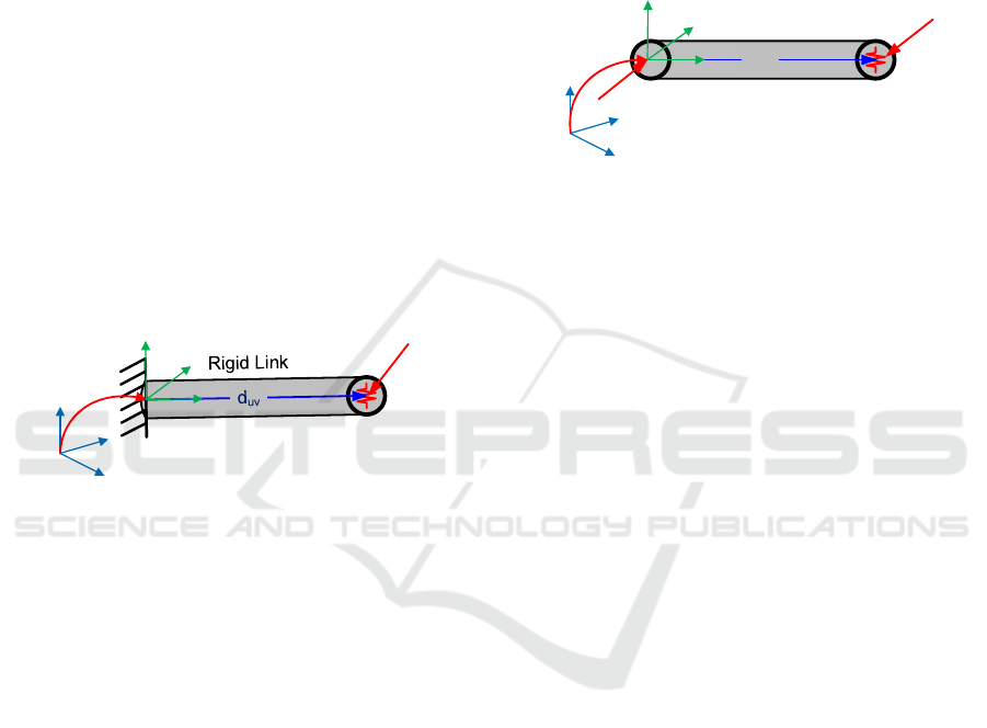
2.1 Stiffness Model of an Elastic Link

VJM represents each elastic component as a

superposition of a rigid element (between the nodes

uv→

), which describes the geometry of the perfect

component, and an elastic component at the right end

of the link (node v), which represents the mechanical

flexibility of the corresponding body, as shown in 0,

where the node u is fixed to the base or previous

component. This model is mathematically expressed

as a linear matrix equation.:

u

v

Δt

uv

R

uv

K

W

Figure 1: VJM-based stiffness model of a flexible link.

uv

=⋅ΔWK t (1)

relating the 6-dimensional wrench

W

consisting of

three force components and three moment

components applied to node v and the corresponding

displacement

Δt

is a 6-dimensional vector

consisting of three linear displacements and three

angular displacements. Here,

66×

stiffness matrix

uv

K must be expressed in the global coordinate

system, while the VJM usually operates with the

stiffness matrix

θ

K

obtained in the local coordinate

system. The latter demands a relevant transformation

θ uv

→KK

33 33

66 66

θ

uv uv

uv

uv u

T

v

××

⋅



=





⋅

R0 R0

KK

0R 0R

(2)

depending on the

33×

rotation matrix

uv

R which

defines the link uv orientation with respect to the

global coordinate system. It should be noted that in

classical VJM, the transformation (2) is incorporated

in the manipulator Jacobian, but it should be applied

straightforwardly here.

Let us also present an alternative MSA-based

model describing the elastic member composed of the

rigid link and virtual spring, assuming that both ends

of the link u, v are not fixed (see 0). Generally, such

a model is represented in the form of a matrix

equation as

d

uv

u

v

Rigid Link

uv

R

v

W

uv

K

v

Δt

u

W

u

Δt

Figure 2: MSA-based stiffness model of a flexible link.

11 12

21 22

1122

uu

vv

×



Δ





=⋅







Δ







Wt

KK

Wt

KK

(3)

relating the 6-dimensional wrenches

()

,

uv

WW

applied to the nodes u, v and the corresponding

displacements

()

,

uv

ΔΔtt

. It is clear that for the

considered physical model (rigid link + virtual

spring), the sub-matrices

11 12 21 22

,,,KKKK

can be

expressed via the spring stiffness matrix

uv

K and link

geometry vector

uv

d . Corresponding derivations are

presented in (Klimchik, Pashkevich, et al., 2019) and

yield the following expression with a symmetrical

matrix of the size

12 12×

1

12 12

TT

u uvuvuv uvuv u

vv

uv uv uv

−−−

−

×



−





=⋅







−







KK

K

WDDD Δt

K

WΔt

D

(4)

It includes

66×

geometric transformation matrix

(Klimchik et al., 2024)

()

3

6

3

333

6

uv

uv×

××

×

 − 

=





×

D

Id

0I

(5)

defining translation from the node u to the node v

expressed in the global coordinate system, which

includes a

33×

skew-symmetric matrix

()

uv

×d

derived from the vector

uv

d (

uv→

) in the following

way

()

31

33

0

0;

0

zy

x

zx y

yx

z

dd

d

dd d

dd

d

×

−





−





=−=−







−







×dd

, (6)

Î

ˇ

T-Y Transformations in Manipulator’s Stiffness Analysis

73

as well as

33×

identity and zero matrices

3333

,

××

I0

. It has been proven that the matrix

uv

D inversion

leads to a simple change of the vector

uv

d direction

()

3

1

3

3333

uv

×

−

×

× 

=





Id

0I

D

(7)

that yield the following properties

1

vu uv

−

=DD

(8)

Similar properties are observed in the transformed

matrices

()

33

3

33

3

33

T

uv

T

uv

××

×

−

×



=







=



−



×

D

I0

dI

I0

dI

D

(9)

Based on these properties, the following important

matrix multiplication rules were derived

11

;

TT T

ij ik kj ik ij kj

−− −−

==DD D DD D

(10)

which are convenient for the mathematical

derivations presented below. It is also worth

mentioning that in eq. (4) the rank of

12 12×

matrix

is equal to 6, which is in good agreement with the

physical properties of link representations. In fact, the

lines of this block matrix are linearly dependent and

satisfy an obvious relation

61

T

uuvv

−

×

+=WDW0

(11)

that in the adopted notation expresses the static

equilibrium condition, resulting in a rank deficiency

of 6. In the following subsection, the obtained model

will be used to derive stiffness models of complex

structures.

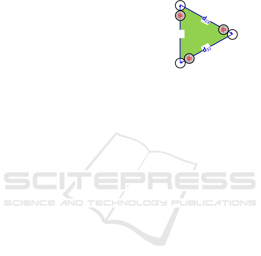
2.2 Stiffness Models of Δ-Structures

Using the elastic link stiffness model (4) let us derive

the stiffness models for Δ- and Y-structures, which

are presented in 0. Each of them consists of three

elastic components connected either at the corners or

a single central node.

2

3

1

K

12

K

23

K

31

d

12

Figure 3: VJM-based stiffness models for Δ-structure and

their parameters.

For the Δ-structure, the stiffness model of the

separate elastic links (1,2) (2,3) (3,1) can be written

as follows:

(12) 1 (12)

1 121212 1212 1

(12) 1 (12)

21212122

TT−−−

−



  

−

=⋅



  

−



  

WKDDD Δt

WD ΔKt

K

(12)

1(23) (23)

23 23 23 23 2322

(23) (23)

1

3323 23 23

TT−−−

−







−

=⋅







−





DDD

W

KK

Δt

WΔtD

(13)

1

(31) (31)

31 31 31 31 31

33

1

(31) (31)

31 31 31

11

TT−−−

−







−

=⋅







−







DDDWK K

KK

Δt

DWΔt

(14)

Further, taking into account that total wrenches

123

,,WWW

are expressed as

(12) (31)

11 1

(12) (23)

22 2

(31) (23)

33 3

=+

WW W

(15)

and the node displacements satisfy the following

constraints

(12) (31)

11

(12) (23)

22

(31) (23)

33

=

Δt Δt

(16)

the desired stiffness model can be re-written in the

form of a single matrix equation

() () ()

11 12 13

11

() () ()

2212223 2

() (

3

18 1

3

8

)()

31 32 33

ΔΔΔ

×



Δ











=Δ







Δ



 



⋅



KKK

Wt

WKKK t

Wt

KKK

(17)

where

ICINCO 2025 - 22nd International Conference on Informatics in Control, Automation and Robotics

74

()

11 12 31

()

12

()

13

()

21

()

22 23 1

1

2

()

23

()

31

()

32

()

33 31 23

1

12 12

1

31 31

1

12 2

1

23 23

31 31

1

23 23

1

31 31

T

Δ− −

−

−−

−

Δ

−−

Δ

+

−

+

−

=

−

=

−

+

=

KKK

KK

KKK

KK

K

DD

D

K

KK

DD

D

K

D

(18)

It can be proved that the rank of

18 18×

matrix is

equal to 12, which agrees with the physical properties

of the considered Δ-structure. In fact, the lines of this

block matrix are linearly dependent and satisfy an

obvious relation

1122 31361

TT−

×

++=WDW DW 0

(19)

that in the adopted notation expresses the static

equilibrium condition, resulting in a rank deficiency

of 6.

2.3 Stiffness Models of Y-Structures

For the Y-structure, presented in 0, the stiffness

model of the separate elastic links (1,0) (2,0) (3,0) can

be written as follows

0

2

3

1

K

30

K

10

K

20

Figure 4: VJM-based stiffness models for Y-structure

and their parameters.

1(10) (10)

10 10 10 10 1011

(10) (10)

1

0010 10 10

TT−−−

−



 

−

=⋅



 

−

 

DDD

W

KK

Δt

WΔtD

(20)

1

(20) (20)

20 20 20 20 20

22

(20) (20)1

0020 20 20

TT−−−

−

 

−

=⋅

 

−

 



DDDWK K

KK

Δt

WΔt

D

(21)

(30) 1 (30)

330303030303

(30) 1 (30)

03030300

TT−−−

−

 

−

=⋅

 

−

 

WKDDD Δt

WD ΔKt

K

(22)

Further, taking into account that total wrenches

123

,,WWW

are expressed as

(10) (20) (30)

00 0 0

(10)

11

(20)

22

(30)

33

=++

=

WW W W

WW

(23)

and the node displacements satisfy the following

constraints

(10) (20) (30)

000

==Δt Δt Δt

(24)

the desired stiffness model can be rewritten in the

form of a single matrix equation

(Y0) (Y0)

11 6 6 14

11

(Y0) (Y0)

2622624 2

(Y0) (Y0)

33

6 6 33 34

(Y0) (

4

66

6

4

6

Y0) (Y0) (Y0)

0

142 344

6

0

××



Δ











Δ



=⋅





Δ









Δ











K00K

Wt

W0K0K t

Wt

00KK

Wt

KKKK

(25)

where

(Y0)

11 10

(Y0)

14

(Y0)

2

3

220

(Y0)

24

(

1

10 10

1

20 20

1

30 30

1

10 10

1

20 20

1

030

10 20 30

Y0)

33 30

(Y0)

34

(Y0)

41

(Y0)

42

(Y0)

43

(Y0)

44

T

−−

−

−−

−

−−

−

=

=++

−

DD

D

DD

D

DD

KK

D

K

D

KK K

(26)

It can be proved that the rank of

24 24×

matrix is

equal to 18, which agrees with the physical properties

of the considered Y-structure. In fact, the lines of this

block matrix are linearly dependent and satisfy an

obvious relation

010120230361

TT T

×

++ + =WDWDWDW0

(27)

the desired stiffness model can be rewritten in the

form of a single matrix equation

To simplify further derivations, let us present both

models in a similar way, with the matrices of the same

dimensions of

18 18×

. For this purpose, let us

eliminate the redundant variable

0

Δt from the linear

matrix equation (25). Taking into account that in the

Î

ˇ

T-Y Transformations in Manipulator’s Stiffness Analysis

75

Δ-type structure, no wrench is applied to the node #0,

i.e.

016×

=W0, the last line of (25) can written as

11 1

10 10 20 20 30 30

10 20 30

123

0

()

−− −

−

Δ

−⋅Δ ⋅ −Δ⋅Δ+

+++⋅=

KtKtKt

KKK t0

DDD

(28)

which yields the following expression for the

deflections in the free node #0

3

11

10 10 2

11

012

1

020

1

30 30

−−−

ΣΣ

−

Σ

−

Δ= Δ+ Δ

Δ+

KD D

D

tK tKK t

KK t

(29)

where

10 20 30Σ

=++KKKK

(30)

After substitution

0

Δt into the three remaining

lines of the equation (25), one can obtain the reduced-

size stiffness model of the Y-structure as

(Y) (Y) (Y)

11 12 13

11

(Y) (Y) (Y)

2212223 2

(Y) (Y) (Y)

33

31 3

18 1

2

8

33

×



Δ

 



 

=Δ



 

Δ



 



⋅



KKK

Wt

W KKK t

Wt

KKK

(31)

where

(Y) 1

11 10

(Y) 1

12

(Y) 1

13

(Y) 1

21

(Y) 1

22 20

(Y) 1

23

(Y)

11

10 10 10 10 10 10

1

10 10 20 20

1

10 10 30 30

1

20 20 10 10

11

20 20 20 20 20 20

1

20 20 30

31

30

TT

T

TT

T

−−− −

−−

−−− −

−

Σ

−

Σ

−

Σ

−

Σ

−

Σ

−

Σ

−

=

KK KKK

KKKK

KK KKK

DDD D

DD

K

D

DK

K

D

K

DD

K

D

1

30 30 10 10

1

30 30 20 20

11

30 3

(

0

1

(Y) 1

3

0

2

Y) 1

33 3 3 30 30 300

T

TT

−−

−

Σ

−

Σ

−− −

Σ

=−

−

=

DD

D

KKK

KK

KDD D

KK

KK KK

(32)

It gives a representation for the Y-structure similar to

the Δ-type one (17). It is obvious that both

representations operate with symmetrical matrices of

size

18 18×

whose rank is equal to 12. Here, the rank

deficiency of 6 is induced by the equilibrium

condition (27), which for

016×

=W0 can be easily

transformed into the form (19) after left-

multiplication by

10

T−

D

and relevant transformations

using the

D-matrix properties (10).

2.4 Transformation of Y-Structure to

Equivalent Δ-Structure

Now, let us derive expressions relating the parameters

of Y- and Δ-structures with similar stiffness

properties (see 0). To derive the desired expressions

for

Y →Δ

transformation, let us equate the upper

off-diagonal components from equations (17) and

(31), i.e. block-matrix elements

() (Y)

12 12

() (Y)

13 13

() (Y)

23 23

Δ

=

KK

(33)

This yields the following equations

1

12 12 10 10 20 20

1

23 23 20 20 30 30

11

31 3 0

1

1 10 1 30 30

TT

T

−− −

Σ

−− −

−

Σ

−

Σ

−

=

−

−−

=

KKKK

KK

DD D

DDKDK

(34)

2

3

1

0

2

3

1

K

30

K

10

K

20

Δ -type model

Y-type model

K

12

K

23

K

31

d

12

Figure 5: VJM-based Y-Δ transformation in the stiffness

models.

that are easily solved for the desired Δ-structures

parameters

12 23 31

,,KKK (stiffness matrices)

1

12 12 10 10 20 20

1

23 23 20 20 30 30

1

31 10 10 30 30 31

1

TT

T

−−

−

Σ

−

Σ

−

Σ

−−

=

KKKK

KK

DD D

DD

K

KKKD

K

(35)

Further, taking into account the symmetry of the

stiffness matrices

jij

T

i

=KK

and specific properties

of the

D-matrix (10) allowing following

simplifications

12 10

23 20

11

10 30 31

20

30

T

TTT

TT

−−

−

=

DDD

D

DD

(36)

the above expressions (35) are reduced to a more

convenient form

11

12 20 10 20 20

11

23 30 20 30 30

11

31 10 30 10 10

T

−−−

Σ

−−−

Σ

−−−

Σ

=⋅ ⋅

KDKKKD

(37)

ICINCO 2025 - 22nd International Conference on Informatics in Control, Automation and Robotics

76

In an alternative way, expressions (37) can be

rewritten with respect to compliances and presented

as

()

1

11111

12 20 10 20 20 10 20

11111

23 30 20 30 30 20 30

11111

31 10 10 30 10 30 10

30

0

20

T

−−−−−

− −−− −

=++

KDKKKKKD

K DKKKKKD

(38)

which are similar to expressions from electrical

engineering, where the resistance corresponds to the

compliance matrices and relevant transformation

equations from Y to Δ circuits are expressed as

follows.

10 20

12 10 20

30

20 30

23 20 30

10

30 10

31 10 30

20

RR

RRR

R

RR

RRR

R

RR

RRR

R

=++

(39)

where

12 23 31

,,RRR

are the Δ-circuit resistances and

10 20 30

,,RRR

are the resistances for the Y-circuit.

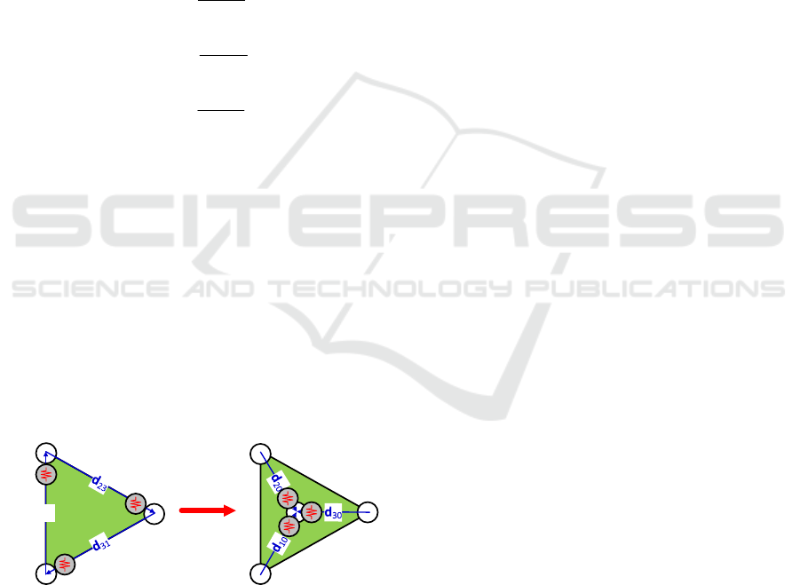
2.5 Transformation of Δ-Structure to

Equivalent Y-Structure

For the inverse transformation, for

YΔ→

transformation (see 0), let us consider the above-

derived equations (37) but solve them for

10 20 30

,,KKK. For convenience, these equations can

be rewritten as

2

3

1

0

2

3

1

K

30

K

10

K

20

K

12

K

23

K

31

d

12

Y -type model

Δ-type model

Figure 6: VJM-based Δ-Y transformation in the stiffness

models.

0

10 20 30

12

1

20 12 20 10 20

1

30 0030

10 20 31

23 30 20 30

1

10 31 10 0 30

()

T

−

=++

DKD K K K K K

(40)

and further transformed to.

10 20 30

10 20 3

11

10 20 12 20 20

11

20 3

0

02330 30

11

30 10 31 10

0

10 20 310

T

−−−

=++

KDKD K K K K

KDKDK K K K

(41)

which yields the following equalities.

11 11

10 20 12 20 20 20 30 23 30 30

11 11

20 30 23 30 30 30 10 31 10 10

11 11

10 20 12 20 20 30 10 31 10 10

TT

−−− −−−

=

KDKD K KDKD K

KDKDK KDKDK

KDKD K KDKD K

(42)

Then, using the first and third relations, the symmetry

of the stiffness matrices

ij

K

as well as commutativity

of the above matrix products, and applying

transposition, one can get expressions

11 11

10 20 12 20 20 30 30 23 30 20

11 11

20 20 12 20 10 30 10 31 10 10

TT

−−− −−−

⋅= ⋅

KDKD K KDKD K

(43)

allowing the derivation of relations between

10 20 30

,,KKK as

11

10 20 12 20 30 23 30 30

11

20 20 12 20 10 31 10 30

TT

−−−

=⋅

KDKDDKDK

(44)

Which using properties (10) can be further simplified

down to

1

10 20 12 23 23 30 30

1

20 20 12 21 31 10 30

TT

−−

=⋅

KDKDKDK

(45)

Substituting these relations into the third relation of

the original system (41) and

11

0

1

20 12 21 31 10 30 30 23 30 30

1

20 12 23 23 30 30

1

20 12 21 31 1 0 303

TT T

TT

−− − −−

−−

⋅=

=⋅+

+⋅+

DKDKD KDKD K

DKDKD K

DKDKD K K

(46)

After executing relevant simplifications, one can

obtain the desired solution for the stiffness matrix

30

K in the form

30 10 31 10 30 23 30

11

30 23 30 20 12 20 10 31 10

TT

TTT−−−

=++

+⋅ ⋅

KDKDDKD

DKD DKD DKD

(47)

Which can also be presented as

000010

30 31 23 23 12 31

−

=++⋅⋅K K K KKK

(48)

which operates with the modified stiffness matrices

of Δ-structures

000

12 23 31

,,KKK

obtained from the

original once

12 23 31

,,KKK

by shifting the reference

point to node #0 in accordance with

Î

ˇ

T-Y Transformations in Manipulator’s Stiffness Analysis

77

0

12 20 12 20

0

23 30 23 30

0

31 10 31 10

T

=

KDKD

(49)

Let us now consider relations (1) and (2) in the system

(42), and using the symmetry of the stiffness matrices

ij

K

as well as the commutativity of the above matrix

products, and applying transposition, one can get the

following expressions

11 11

10 20 12 20 20 30 30 23 30 20

11 11

20 30 23 30 30 10 10 31 10 30

TT

−−− −−−

⋅= ⋅

KDKD K KDKD K

(50)

allowing the derivation of relations between

10 20 30

,,KKK as

11

30 30 23 30 20 12 20 10

11

20 30 23 30 10 31 10 10

TT

−−−

=⋅

KDKDDKDK

(51)

Which using properties (10) can be further simplified

down to

1

30 30 23 32 12 20 10

1

20 30 23 31 31 10 10

TT

−−

=⋅

K DKDKD K

KDKDKDK

(52)

Substituting these relations into the third relation of

the original system (41) and executing relevant

simplifications, one can obtain the desired solution

for the stiffness matrix

30

K in the form

10 20 12 20 10 31 10

11

10 31 10 30 23 30 20 12 20

TT

TTT−−−

=++

+⋅ ⋅

KDKDDKD

DKD DK D DKD

(53)

Which can also be presented as

000010

10 12 31 31 23 12

−

=++⋅⋅K KKKKK

(54)

In a similar way, the expressions can also be derived

for

20

K

20 30 23 30 20 12 20

11

20 12 20 10 31 10 30 23 30

TT

TTT−−−

=++

+⋅ ⋅

KDKDDKD

DKD DKD DKD

(55)

Or in the form

000010

20 23 12 12 31 23

−

=++⋅⋅KKKKKK

(56)

Hence, the final solution has the following

presentation

000010

10 12 31 31 23 12

000010

20 23 12 12 31 23

000010

30 31 23 23 12 31

−

=++⋅⋅

KKKKKK

(57)

Also, after relevant matrix transformations and

inversion of eq. (57), the desired solutions can be

presented with respect to the compliance

()

1

101010101 01

10 12 12 23 31 31

1

1 0 10 10 10 1 0 1

20 23 12 23 31 12

1

101010101 01

30 31 12 23 31 23

−

− −−−− −

−

−−−−− −

−

− −−−− −

=++

K KKKK K

KKKKK K

K KKKK K

(58)

Thus, the obtained expressions (37), (38), (57) and

(58) allow the transformation of the Y-type elastic

structure into the equivalent Δ-type one and vice

versa. They are similar to the scalar expressions from

electrical engineering.

12 31

10

12 23 31

12 23

20

12 23 31

23 31

30

12 23 31

RR

R

RRR

RR

R

RRR

RR

R

RRR

=

++

=

++

=

++

(59)

However, the expressions for stiffness

transformations are based on the

66×

matrix

operations and include additional components

ij

D

that take into account the geometry of the relevant

mechanical structure, although they can be excluded

if all stiffness matrices

ij

K

are presented with respect

to the node #0, i.e. in the form

0

ij

K

defined by eq.

(49). It is worth mentioning that for

YΔ→

transformations, the location of the node #0 can be

assigned arbitrarily. Besides, it should be noted that

because of the symmetry of the matrices

ij

K

and

0

ij

K

leading to commutativity of some matrix

products, one can obtain slightly different expressions

for equivalent stiffness/compliance matrices, which

are equal up to a transposition.

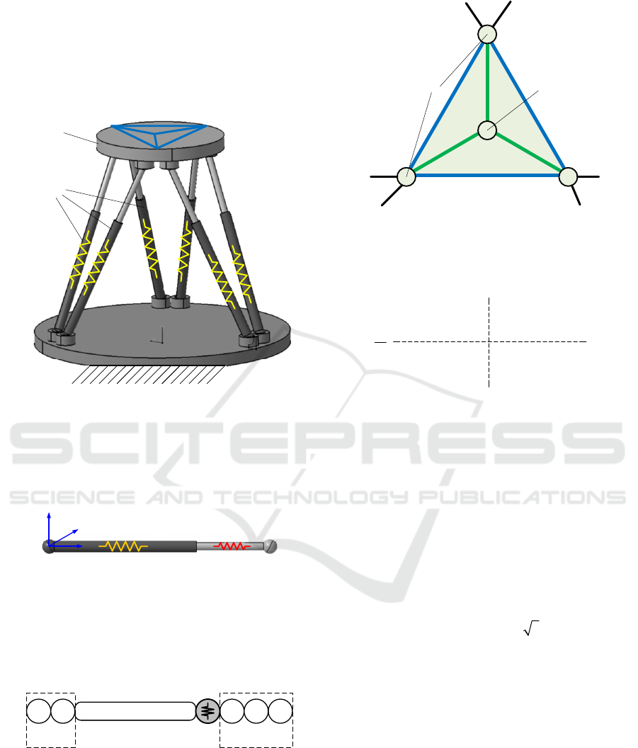
3 APPLICATION EXAMPLE

To demonstrate the value of the proposed technique,

let us apply it to the stiffness analysis of the Gough-

Stewart manipulator with a non-rigid mobile platform

(see 0). Legs’ stiffness modelling (0) does not create

any problems due to their strictly serial kinematics

(Klimchik

et al., 2012). However, due to the

platform's elasticity, the entire mechanism cannot be

presented as a serial-parallel structure, as is typically

considered in relevant works. In fact, the platform

contains multiple elastic cross-linkages that make it

ICINCO 2025 - 22nd International Conference on Informatics in Control, Automation and Robotics

78

impossible to handle within the frame of the

conventional VJM approach. However, using the

developed

YΔ→

transformation, one can obtain an

equivalent pure serial-parallel topology suitable for

stiffness modelling employing the VJM approach.

Elastic

platform

Elastic

Legs

Figure 7: Gough-Stewart platform with 3-3 connection.

The considered elastic platform consists of six

mutually connected elastic beams forming the frame,

as shown in 0. For each beam, the

66×

the stiffness

matrix is computed using the following expression

Rigid Link R

z

R

x

R

y

R

y

R

z

U-joint S-joint

6-d.o.f.

spring

x

z

y

U-joint

(passive)

S-joint

(passive)

{R

x

} {R

y

} {R

z

}

{R

y

}

{R

z

}

P-joint

(actuated)

{T

x

}

(b) VJM-based model of Gough-Stewart leg

(a) kinematic model of Gough-Stewart leg

Figure 8: VJM-based stiffness models for Gough-Stewart’s

leg.

Leg #1

Leg #2

Leg #3 Leg #4

Leg #5

Leg #6

Reference

point

Connection

joints

Figure 9: Gough-Stewart’s Δ+Y structure of mobile

platform.

2

44

2

3

0000 0

012 0 0 0 6

001206 0

00 0 0 0

006 04 0

06 00 04

zz

yy

beam

yy

zz

A

II

E

L

I

K

I

L

ILI

LL

L









−









=













−









K

(60)

where

2

44

(1 ) / 2KJL

υ

=+

, Young's modulus

E

and

Poisson's ratio coefficient

υ

describe beam’s elastic

properties, its geometry is described by length

L and

cross-section area

A, the variables I

y

, I

z

, and J are the

cross-section quadratic and polar moments of inertia.

For the considered example, it is assumed that

actuated legs are connected to the elastic platform at

the corners of the equilateral triangle with the edge

length

a

, while the reference point is located at the

triangle's centre. For such an arrangement, the lengths

of the links (1,2), (2,3) and (3,1) are equal to the

triangle parameter

a

and the lengths of the links

(1,0), (2,0) and (3,0) are

/3ba= . The remaining

parameters included in the matrix

beam

K are

computed as

2

/4Ad

π

=⋅

,

4

/64

yz

II d

π

==⋅

,

4

/32Jd

π

=⋅

, where d is the link diameter that is

assumed to have a circular cross-section.

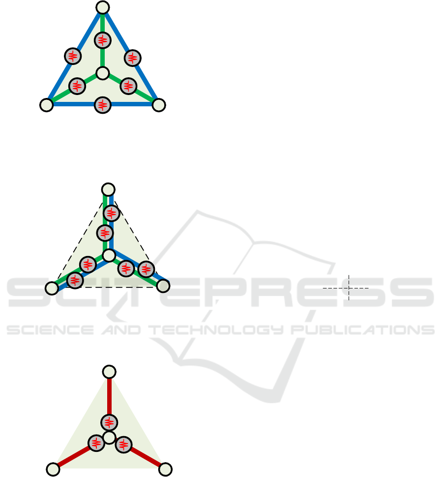
The original platform consisted of six mutually

connected elastic elements: three beams of length

a

and three beams of length

b (0a). After applying the

developed

YΔ→

transformation, the original

model is converted into an equivalent double-Y-

structure composed of six elements of length

b each

(0b). Then this double-Y-structure was transformed

into a classical Y-structure that can be easily handled

by the conventional VJM approach (0c).

Î

ˇ

T-Y Transformations in Manipulator’s Stiffness Analysis

79

2

31

0

d

30

d

20

3

1

2

0

10

′

K

10

′′

K

10

K

20

′′

K

30

′′

K

d

10

d

31

d

23

d

12

10

K

12

K

23

K

31

K

30

′

K

20

K

20

K

20

′

K

30

K

30

K

(a) Original structure of elastic

platform with cross-linkages

(b) Equivalent model for elastic

platform without cross-linkages

(c) Target equivalent Y-type

model for elastic platform

Figure 10: VJM-based stiffness models for the Δ-structure

and their parameters.

Using the developed

YΔ→

transformation, we can

compute

10 20 30

,,

′′′

KKK

as follows

000010

10 12 31 31 23 12

000010

20 23 12 12 31 23

000010

30 31 23 23 12 31

−

′

=++⋅⋅

′

=++⋅⋅

′

=++⋅⋅

KKKKKK

(61)

And then, considering the parallel connection of

10 20 30

,,KKK and

10 20 30

,,

′′′

KKK

get stiffness

matrices

10 20 30

,,

′′ ′′ ′′

KKK

as

10 10 10

20 20 20

30 30 30

′′ ′

=+

′′ ′

=+

′′ ′

=+

KKK

(62)

To obtain the stiffness model for the entire

manipulator, one can consider pairs of legs connected

in parallel and attached to the mobile platform, i.e. we

can write

() 1 2

10

() 3 4

10

() 5 6

10

leg

leg leg

leg

leg leg

leg

leg leg

=+

KKK

(63)

Where leg stiffness matrices

i

leg

K

can be computed

as follows (see (Klimchik

et al., 2025) for details)

33

11

33 33

T

i

ii

leg

K

×

××





⋅

=⋅









uu 0

K

00

(64)

where

11

/KLEA= is the leg stiffness on the

compression along the main axis and

i

u The unit

direction vectors specify the orientation of the leg.

To integrate the legs’ stiffness in the stiffness model

of the manipulator, we need to move

()leg

i

K

to the

zero node using the following transformations

0

(0) 10

10 10

2

10

(0) 20

20

(0) 30

300

20

330

T

i

T

leg leg

=

KK

D

DKK

D

DD

D

(65)

Thus, the final Cartesian stiffness matrix for the

Gough-Stewart Platform can be computed as

()( )

()

(0) (0)

10 10 20 20

(0)

30 30

Cleg leg

leg

′′ ′′

=+ ++ +

′′

++

KKK KK

KK

(66)

Hence, this development expands the application

scope of the VJM method for over-constrained

parallel manipulators, where cross-linkages are

widely used to improve stiffness properties.

ICINCO 2025 - 22nd International Conference on Informatics in Control, Automation and Robotics

80

4 CONCLUSIONS

This paper proposes a new stiffness model

transformation technique for modelling the elastic

behaviour of hybrid over-constrained robotic

manipulators with multiple cross-linkages. This

technique helps users address the critical limitation of

the VJM method. It provides an analytical expression

for equivalent transforming the cross-linkages into

serial-parallel structures suitable for the VJM.

To derive the desired transformations, the specific

MSA-based representation is employed, which uses a

conventional VJM-type

66×

virtual springs. This

helps to derive analytical relations between the

equivalent models. The main results were obtained

for 3-node structures, but they can be further

generalised for the n-node case. To demonstrate the

efficiency of the developed technique, Gough-

Stewart manipulator with elastic platforms and

compliant legs was considered.

ACKNOWLEDGEMENTS

This work was partly supported by French Agence

Nationale de la Recherche (ANR) under reference

ANR-23-CE10-0004-02' (project RAPHy).

REFERENCES

Blumberg, J., Li, Z., Besong, L. I., Polte, M., Buhl, J.,

Uhlmann, E. & Bambach, M. (2021). 26th International

Conference on Automation and Computing, pp. 1-6.

Deblaise, D., Hernot, X. & Maurine, P. (2006). IEEE

International Conference on Robotics and Automation

(ICRA 2006), pp. 4213-4219.

Detert, T. & Corves, B. (2017). New Advances in

Mechanisms, Mechanical Transmissions and Robotics,

edited by B. Corves, E.-C. Lovasz, M. Hüsing, I. Maniu

& C. Gruescu, pp. 299-310. Springer.

Gonzalez, M. K., Theissen, N. A., Barrios, A. & Archenti,

A. (2022). Robotics and Computer-Integrated

Manufacturing 76, 102305.

Görgülü, İ., Carbone, G. & Dede, M. İ. C. (2020).

Mechanism and Machine Theory 143, 103614.

Gosselin, C. & Zhang, D. (2002). International Journal of

Robotics and Automation 17, 17-27.

Hu, M., Wang, H. & Pan, X. (2019). 2019 IEEE

International Conference on Robotics and Biomimetics

(ROBIO), pp. 1653-1658.

Hussain, I., Albalasie, A., Awad, M. I., Tamizi, K., Niu, Z.,

Seneviratne, L. & Gan, D. (2021). IEEE Access 9,

118215-118231.

Kim, S. H. (2023). Journal of Manufacturing Processes 89,

142-149.

Kim, S. H. & Min, B.-K. (2020). International Journal of

Precision Engineering and Manufacturing 21, 1017-

1023.

Klimchik, A., Chablat, D. & Pashkevich, A. (2019). pp.

355-362. Cham: Springer International Publishing.

Klimchik, A., Pashkevich, A., Caro, S. & Chablat, D.

(2012). Robotics, IEEE Transactions on 28, 955-958.

Klimchik, A., Pashkevich, A., Caro, S. & Furet, B. (2017).

2017 IEEE International Conference on Advanced

Intelligent Mechatronics (AIM), pp. 285-290.

Klimchik, A., Pashkevich, A. & Chablat, D. (2018). 12TH

IFAC Symposium on robot control - SYROCO 2018.

Klimchik, A., Pashkevich, A. & Chablat, D. (2019).

Mechanism and Machine Theory 133, 365-394.

Klimchik, A., Pashkevich, A. & Chablat, D. (2025).

Stiffness Modeling of Parallel Robots: Springer.

Klimchik, A., Pashkevich, A., Chablat, D. & Hovland, G.

(2013). Robotics and Computer-Integrated

Manufacturing 29, 385-393.

Klimchik, A., Paul, E., Krishnaswamy, H. & Pashkevich,

A. (2024). 2024 10th International Conference on

Control, Decision and Information Technologies

(CoDIT), pp. 1897-1902.

Klimchik, A., Wu, Y., Dumas, C., Caro, S., Furet, B. &

Pashkevich, A. (2013). IEEE International Conference

on Robotics and Automation (ICRA) pp. 3707-3714.

Majou, F., Gosselin, C., Wenger, P. & Chablat, D. (2007).

Mechanism and Machine Theory 42, 296-311.

Nguyen, V. L., Kuo, C.-H. & Lin, P. T. (2022). Mechanism

and Machine Theory 170, 104717.

Pashkevich, A., Chablat, D. & Wenger, P. (2009).

Mechanism and Machine Theory 44, 966-982.

Pashkevich, A., Klimchik, A. & Chablat, D. (2011).

Mechanism and machine theory 46, 662-679.

Quennouelle, C. & Gosselin, C. á. (2008). Advances in

Robot Kinematics: Analysis and Design, pp. 331-341:

Springer.

Soares Júnior, G. D. L., Carvalho, J. C. M. & Gonçalves, R.

S. (2015). Robotica 34, 2368-2385.

Wu, K., Li, J., Zhao, H. & Zhong, Y. (2022). Applied

Sciences 12, 8719.

Yue, W., Liu, H. & Huang, T. (2022). Mechanism and

Machine Theory 175, 104941.

Zhao, W., Klimchik, A., Pashkevich, A. & Chablat, D.

(2022). Mechanism and Machine Theory 172, 104783.

Î

ˇ

T-Y Transformations in Manipulator’s Stiffness Analysis

81