Solving the Three-Dimensional Beacon Placement Problem Using

Constraint-Based Methods, Large Neighborhood Search, and

Evolutionary Algorithms

Sven L

ofﬂer, Viktoria Abbenhaus, George Assaf and Petra Hofstedt

Department of Mathematics and Computer Science, MINT, Programming Languages and Compiler Construction Group,

Brandenburg University of Technology Cottbus-Senftenberg, Konrad-Wachsmann-Allee 5, Cottbus, Germany

ﬂ

Keywords:

Beacon Placement, Constraint Programming, CSP, COP, Large Neighborhood Search, LNS, Evolutionary

Algorithms, Indoor Positioning, Optimization Algorithms, Decision Support Systems.

Abstract:

With the increasing prevalence of large building complexes, indoor localization is becoming an area of growing

signiﬁcance. In critical situations, such as emergencies in factories or care facilities, the ability to locate a

person quickly can be a matter of life and death. One possibility for localization are Bluetooth beacons, which

are either attached to the person or in rooms. We pursue the latter approach, whereby the beacon signals are

used to determine the position of a receiving device, e.g. a mobile phone. At this, the use of a sufﬁcient

number of beacons in the building must be ensured in order to guarantee adequate coverage. However, to

minimize costs, it is equally important to avoid placing unnecessary beacons. This creates a challenging

optimization problem that this paper addresses through three distinct approaches: constraint programming,

large neighborhood search, and evolutionary algorithms. Using simulated three-dimensional buildings, we

test and evaluate these methods, ultimately providing a practical and efﬁcient approach applicable to real-

world building environments.

1 INTRODUCTION

Both in industrial settings, such as large factories,

and in private residential areas, including dormitories

and care facilities, increasingly large building com-

plexes are being constructed where people work, live,

and may also encounter emergencies. In such situa-

tions, it is critical to locate and assist individuals as

quickly as possible. A viable solution for indoor lo-

calization, which also respects individuals’ privacy,

is the use of Bluetooth beacons. However, to mini-

mize costs, it is essential to deploy the fewest num-

ber of beacons necessary. This creates a signiﬁcant

optimization challenge, heavily inﬂuenced by the ar-

chitecture of the building. Factors such as wall and

window types and thickness, as well as room layouts

and sizes, affect the range of each beacon. For reliable

position detection using triangulation, every point in

the building must be covered by signals from at least

three beacons. This paper examines the challenges of

this problem and provides solutions tailored to diverse

building conﬁgurations.

Indoor localization has a wide range of applica-

tions, including indoor navigation, asset tracking, per-

sonnel monitoring, and more. Common techniques in

indoor positioning algorithms involve Bluetooth Low

Energy (BLE) beacons and signal strength measure-

ments, which are often used for triangulation, trilater-

ation, or proximity-based approaches (Sakpere et al.,

2017; Bembenik and Falcman, 2020). This article fo-

cuses on trilateration, a method for determining the

position of a point based on its distances to three ref-

erence points.

The optimal placement of beacons for trilateration

aims to minimize the number of beacons required (re-

ducing costs) while ensuring seamless coverage of the

space (triple signal coverage of all points). Currently,

beacon placement is often performed manually, which

is not only time-consuming but also prone to errors.

Despite extensive testing, manual methods provide

no guarantees of complete coverage across the entire

building nor certainty regarding the minimum or an

acceptably small number of beacons required.

Our novel approaches, based on constraint pro-

gramming (CP), large neighborhood search (LNS),

and evolutionary algorithms (EA), address this chal-

lenge by guaranteeing full coverage of all posi-

tions with a minimal number of beacons in three-

Löfﬂer, S., Abbenhaus, V., Assaf, G. and Hofstedt, P.

Solving the Three-Dimensional Beacon Placement Problem Using Constraint-Based Methods, Large Neighborhood Search, and Evolutionary Algorithms.

DOI: 10.5220/0013724500003982

Paper published under CC license (CC BY-NC-ND 4.0)

In Proceedings of the 22nd International Conference on Informatics in Control, Automation and Robotics (ICINCO 2025) - Volume 1, pages 105-116

ISBN: 978-989-758-770-2; ISSN: 2184-2809

105

dimensional buildings. By adopting a conservatively

chosen set of parameters, our methods ensure reliable

and efﬁcient beacon placement while signiﬁcantly re-

ducing the risks associated with manual approaches.

The remainder of this paper is organized as fol-

lows. Section 2 discusses various existing approaches

for beacon placement. Section 3 provides the foun-

dational concepts of constraint programming, large

neighborhood search, and evolutionary algorithms.

Section 4 describes the proposed methods for deter-

mining an optimized beacon placement. In Section 5,

the different approaches are evaluated in terms of their

applicability and quality across various generated test

buildings. Finally, Section 6 concludes the paper with

a summary of ﬁndings and an outlook on future work.

2 RELATED WORK

This section ﬁrst discusses related work on the topic

of automatic beacon placement, followed by an exam-

ination of our previous research on 2D beacon place-

ment.

2.1 Automatic Beacon Placement

Numerous recent studies have focused on optimizing

beacon placement for indoor positioning, employing

a variety of approaches.

A key aspect of beacon placement is selecting

appropriate metrics to evaluate positioning accuracy.

The Geometric Dilution of Precision (GDOP), origi-

nally developed for satellite navigation systems, has

been successfully adapted for 5G mmWave networks

to optimize base station selection for positioning. In

(Rajagopal et al., 2016), GDOP was adapted for in-

door environments, leading to a signiﬁcant reduction

in the number of beacons required compared to stan-

dard trilateration methods.

Another approach utilizes Time-of-Flight (ToF)

signals between beacons and target devices. (Wang

et al., 2019) investigates beacon position optimization

and proposes a greedy algorithm that initially places

O(OPT ln(m)) beacons. Additionally, a random sam-

pling algorithm is introduced, reducing the required

beacons to O(OPT ln(OPT )), resulting in fewer bea-

cons compared to earlier approaches.

The study by (McGuire et al., 2021) focuses on the

self-localization of autonomous vehicles using Angle-

of-Arrival (AoA) for position calculation, incorporat-

ing course angles. It presents the determinant of the

Fisher Information Matrix for an arbitrary number of

beacons and derives the optimal angular spacing for

three beacons through numerical simulations.

Another approach, proposed by (Sharma and

Badarla, 2018), treats the beacon placement area as

a grid of candidate positions on ceilings and walls. It

minimizes the total number of beacons while adhering

to GDOP constraints using Mixed Integer Linear Pro-

gramming (MILP). This method improves the mini-

mum GDOP without increasing the number of bea-

cons.

To our knowledge, no other work has imple-

mented a comparable constraint-programming-based

approach for beacon placement exclusively using

Boolean variables. Furthermore, known methods are

designed for two-dimensional spaces, whereas we

aim to extend these approaches to three-dimensional

environments. Transitioning to three-dimensional

space introduces a critical challenge: the lack of scal-

ability of certain algorithms. The addition of a third

dimension signiﬁcantly increases the search space,

often preventing many algorithms from ﬁnding sufﬁ-

ciently good solutions within acceptable timeframes.

2.2 Prior Work by the Authors

In this subsection, we present our previous contribu-

tions to the ﬁeld of optimal beacon placement (L

ofﬂer

et al., 2022). Our prior work has primarily focused on

constraint-based two-dimensional beacon placement

strategies, laying the foundation for the advancements

discussed in this paper.

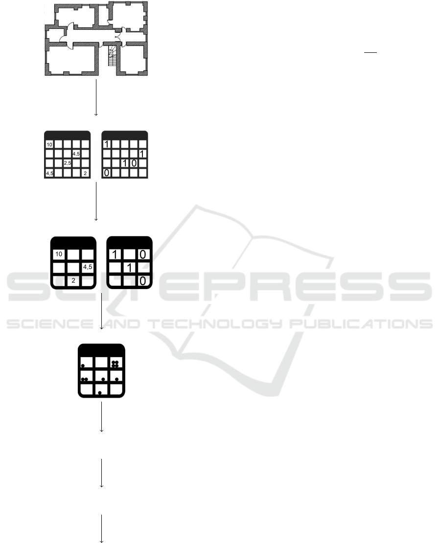
Figure 1 provides an overview of the approach

used to compute an optimal beacon placement as de-

scribed in (L

ofﬂer et al., 2022). The process begins

by importing an image of a ﬂoor plan, which is then

preprocessed into two 2D arrays: an environmental

resistance array A

and a reachability array A

The environmental resistance array A

encodes

environmental factors E corresponding to materials in

the map. These factors were determined experimen-

tally as follows: E(open spaces) = 2, E(drywall) =

2.5, E(solid walls) = 4.5, and E(glass) = 10.

The reachability array A

is a Boolean array where

the entry at position (x, y) indicates whether the corre-

sponding location (x, y) must be triple-covered by the

beacons (True) or not (False). The latter case applies,

for instance, to areas outside the building or regions

blocked by thick walls.

In the next step, both arrays are scaled, aggregat-

ing the pixels of the original map into larger pixel

blocks. This process is performed conservatively,

meaning the aggregated pixel blocks adopt the maxi-

mum environmental resistance E of their constituent

pixels, and any block remains reachable if even one

of its original pixels was reachable.

Using an RSSI-based distance calculation (see

ICINCO 2025 - 22nd International Conference on Informatics in Control, Automation and Robotics

106

Map of the building

2-D env. resistance A

and reachability arrays A

Preprocessing

Scaled env. resistance A

and reachability arrays A

Different scalings s = 4, 5, 10, 15, ..., 54, 60

Beacon coverage set S

RSSI based range calculation

Scaled COP

COP construction

P = (X, D,C, min(numOfBeacons))

Optimized COP

COP reﬁnements

opt

= (X, D,C, min(numOfBeacons))

Beacon positioning

COP solving

Figure 1: Overview of the beacon positioning process from

ofﬂer et al., 2022).

Equation 1, (Li et al., 2018)), the potential coverage

of a beacon placed at position (x, y) is determined.

Speciﬁcally, for each position (x, y), the set of all po-

sitions covered by a beacon at that location is calcu-

lated, forming a coverage set S.

distance = 10

−

RSSI

10∗E

(1)

Subsequently, a constraint optimization problem

(COP) P is formulated based on these coverage sets.

The COP P is then further optimized through var-

ious reﬁnements to P

opt

for runtime efﬁciency and

solved globally to determine an optimal beacon place-

ment. Among these reﬁnements, parallelization meth-

ods (parallel portfolio (R

egin and Malapert, 2018))

and the addition of extra constraints were considered.

Figure 2 depicts an example section of a ﬂoor plan

with scaled pixels overlaid. The different wall types

are represented by green (drywall with E=2.5), blue

(solid wall with E=4.5), and red (glass with E=10),

with varying wall thicknesses. These characteristics

result in different signal ranges for individual bea-

cons. Using the previously introduced method, the

original pixels are scaled into the deﬁned scaled pix-

els. This means that any scaled pixel containing walls

is assigned the signal resistance value of the highest

resistance present within it. For example, the scaled

pixel in row 2 and column 3 contains free space (E =

2), a drywall (E = 2.5), and a glass wall (E = 10), re-

sulting in a scaled glass pixel with E = 10 (see Figure

3). Additionally, the accessibility of the scaled pix-

els must be deﬁned. In Figure 2, it is assumed that

areas containing walls are not required to be triple-

covered by beacon signals. However, in the scaled

version shown in Figure 3, this means that scaled pix-

els with at least one accessible original pixel must

remain accessible (Non-accessible areas are marked

with hatched patterns in the ﬁgure). An example of

such a pixel that must remain accessible, even if parts

of the original pixels are walls, is the pixel located in

row 2, column 3.

The scaled pixels, represented in the algorithm

process (see Figure 1) by the arrays A

and A

, serve

as the foundation for the subsequent constraint prob-

lem, which calculates the optimal beacon placement.

In Figure 3, multiple beacons (B) are shown, forming

part of a solution that ensures triple coverage of the

entire accessible building while minimizing the num-

ber of beacons used.

In (L

ofﬂer et al., 2023), we introduced an alter-

native approach based on set variables to model and

solve the constraint problem. Compared to the ap-

proach presented in (L

ofﬂer et al., 2022), this method

achieved solutions slightly faster but at the cost of re-

duced solution quality. Since the quality of the solu-

Solving the Three-Dimensional Beacon Placement Problem Using Constraint-Based Methods, Large Neighborhood Search, and

Evolutionary Algorithms

107

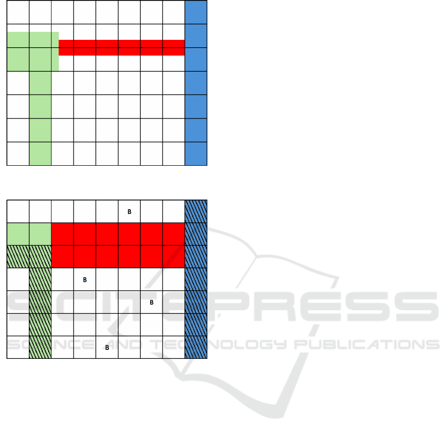
Figure 2: A section of a building ﬂoor plan for a single ﬂoor,

shown in top-down view, with a scaled pixel grid.

Figure 3: A scaled section of a building ﬂoor plan for a

single ﬂoor with a random distribution of beacons.

tion is of primary importance for our objectives, we

have decided to proceed with the ﬁnite-domain ap-

proach from (L

ofﬂer et al., 2022) in the present work.

However, given the modular design of methodology

presented below, it could also be adapted to use the

set-variable-based approach if desired.

However, both methods are tailored to two-

dimensional spaces. Extending the approach to three-

dimensional spaces introduces signiﬁcant challenges,

as the constraint model becomes excessively large and

computationally expensive. This paper addresses this

limitation by proposing novel methodologies that ef-

ﬁciently handle the increased complexity and scala-

bility requirements of three-dimensional spaces.

3 PRELIMINARIES

In this section, we provide an overview of the fun-

damental principles underlying Constraint Program-

ming, Large Neighborhood Search, and Evolutionary

Algorithms.

3.1 Constraint Prgramming

Constraint Programming (CP) is a powerful declar-

ative approach for modeling and solving NP-hard

problems. Common research domains in CP include

rostering, graph coloring, optimization, and satisﬁa-

bility problems (SAT) (Marriott, 1998). Using con-

straint programming, a global optimum can be found

and validated, which typically makes this approach

highly time-consuming. The general CP workﬂow

can be divided into two main components: 1. the

declarative respresentation as a constraint model, 2.

solving the constraint model using an independent

solver.

A Constraint Satisfaction Problem (CSP) is for-

mally represented as a triple P = (X, D,C), where:

X = {x

, x

, . . . , x

} is a set of variables, D =

, D

, . . . , D

} is a set of ﬁnite domains, where D

is the domain of variable x

, and C = {c

, c

, . . . , c

}

is a set of constraints that may involve one or more

variables from X (Apt, 2003a). A constraint is a tuple

(X, R), where X is an ordered set of variables and R is

a relation deﬁned over X (Dechter, 2003a).

A solution of a CSP is an instantiation of all vari-

ables x

with values d

∈ D

such that all constraints

are satisﬁed. A Constraint Optimization Problem

(COP) extends a CSP by introducing an objective

variable x

opt

, which must be either minimized or max-

imized.

For this work, a critical constraint is the count

constraint. The count(X, occ, v) constraint restricts

the variables in set X such that the value v occurs

exactly occ times (Demassey and Beldiceanu, 2024;

van Hoeve and Katriel, 2006). An example of the

count constraint is count({x

, x

}, {1, 3}, 2) with

= d

= {1, 2, 3}. In this case, the value 2

must appear exactly one or three times in the vari-

ables x

, x

. Possible solutions include, for in-

stance, x

= 1, x

= 2, x

= 3 or x

= 2, x

= 2.

CSPs and COPs are typically solved using a back-

tracking search algorithm combined with constraint

propagation. Popular solvers for ﬁnite domain prob-

lems include Google OR-Tools (Perron and Furnon,

2023), Gecode (Christian Schulte, 2019), and Choco-

Solver (Prud’homme and Fages, 2022), with the lat-

ter being utilized in this work. For more detailed in-

formation on solvers and their mechanisms, see (Apt,

2003b; Dechter, 2003b; Rossi et al., 2006).

ICINCO 2025 - 22nd International Conference on Informatics in Control, Automation and Robotics

108

3.2 Large Neighborhood Search

Large Neighborhood Search (LNS) was ﬁrst intro-

duced in (Shaw, 1998) as a method for solving big

constraint problems. This approach involves destroy-

ing a signiﬁcant portion of the variable assignments in

a given solution, followed by an optimization step to

repair the solution and potentially ﬁnd a better one.

This approach can typically only determine locally

optimal solutions. The original work focuses on solv-

ing the Vehicle Routing Problem (VRP). In this pa-

per, we adapt the method for the optimal placement

of beacons.

The core idea behind the destruction phase is to

modify or remove parts of the current solution based

on a heuristic. In the context of a constraint problem,

this means reversing variable assignments, effectively

freeing those variables to take on new values from

their respective domains.

During the repair phase, the resulting partial struc-

ture is reﬁned using an optimization technique, such

as constraint programming or local search methods.

The rationale is that the original CP model is often too

large and complex to be solved globally in a reason-

able amount of time. By partially destroying the com-

plete solution, a smaller subproblem is created that is

computationally more tractable. This subproblem can

then be solved to global optimality. However, solv-

ing the subproblem globally does not imply a global

solution to the original problem.

Through iterative cycles of destruction and repair,

the algorithm aims to escape local optima and pro-

gressively approach a global solution (without guar-

antee that this will be achieved). This strategy lever-

ages the balance between exploration and exploita-

tion, allowing the method to effectively navigate the

solution space.

3.3 Evolutionary Algorithms

Inspired by Darwin’s understanding of evolution

(Darwin, 1859), algorithms have been developed to

mimic this process computationally. The fundamen-

tal idea is that an environment can sustain only a lim-

ited number of individuals. However, each individual

possesses an inherent drive for reproduction, neces-

sitating a selection process based on the principle of

”survival of the ﬁttest.”

Each individual represents a unique combination

of phenotypic traits, which are evaluated by the envi-

ronment. If this combination is favorable, the individ-

ual has a higher probability of producing offsprings.

Darwin’s key insight was that small, random varia-

tions (mutations in phenotypic traits) occur naturally

during reproduction, passing from one generation to

the next. Even though this approach allows for the

simultaneous consideration of multiple solutions, it

typically still results in only locally optimal solutions.

Algorithm 1: Evolutionary Algorithm.

Data: Population size n, crossover rate r

mutation rate r

, max generations g

Result: Best individual found during the

evolution process

1 P = generatePopulation(n)

2 for i = 1 to g do

3 P

′

= crossover(P, r

)

4 P

′

= mutate(P

′

, r

)

5 P = survivorSelection(P, P

′

, n)

6 end

7 return best(P)

Algorithm 1 outlines the procedure of an evolu-

tionary algorithm (Popyack, 2016). Initially, a pop-

ulation of n random individuals is generated (line 1).

As long as the maximum number of generations g has

not been reached (line 2), a crossover operation is per-

formed between two or more individuals, depending

on the crossover rate r

(line 3). Typically, individuals

with higher ﬁtness values are preferentially selected

for crossover.

Following the crossover, the resulting offspring

undergo mutation based on the mutation rate r

which involves introducing random changes to cer-

tain values of an individual (line 4). This enhances

genetic diversity within the population.

Subsequently, the new population P is formed by

selecting the n ﬁttest individuals from the combined

set of the current population P and the newly gener-

ated offspring P

′

(line 5). After g iterations, the algo-

rithm returns the best individual found (line 7).

Typical application areas of evolutionary algo-

rithms include optimization problems (Slowik and

Kwasnicka, 2020), such as ﬁnding optimal model pa-

rameters in machine learning (Shanthi and Chethan,

2023).

4 MODELING THE PROBLEM

In this section, we ﬁrst describe our representation of

the three-dimensional space of buildings using pixels,

before discussing our various solution approaches.

Solving the Three-Dimensional Beacon Placement Problem Using Constraint-Based Methods, Large Neighborhood Search, and

Evolutionary Algorithms

109

4.1 Representation of the 3-D Space

In (L

ofﬂer et al., 2022; L

ofﬂer et al., 2023), we used

two-dimensional n × n pixels to represent the ﬂoor

plan of a single level. Each pixel was assigned one of

the values E = 2, 2.5, 4.5 or 10 to reﬂect the character-

istics of the ﬂoor plan. Larger pixel sizes led to more

pessimistic abstractions, as the worst value within a

pixel’s area was always assumed for the entire pixel.

Extending this representation into a three-

dimensional space by using n × n × n voxels is im-

practical. For instance, with a ceiling-plus-ﬂoor

height of h = 3 meters and a pixel side length of 10

cm, this would result in 30 stacked voxels per ﬂoor.

Consequently, the computation of coverage sets S,

i.e., the beacon ranges, would become signiﬁcantly

more complex for even a single ﬂoor.

Unlike horizontal layouts, where walls can appear

at various positions, ﬂoors and ceilings are gener-

ally uniform in vertical structure. This implies the

presence of a solid ceiling (or ﬂoor) of thickness h

with E = 4.5 (solid wall), which does not need to be

reachable, and beneath it, a space of room height h

This space could be open (E = 2), contain a drywall

(E = 2.5), a solid wall (E = 4.5), or glass (E = 10),

among other possibilities.

To simplify vertical abstraction and considering

that the general beacon range signiﬁcantly exceeds

the ﬂoor height h (room height h

plus ceiling thick-

ness h

), each pixel is assigned dimensions of n × n×

h with h = h

. This allows us to compute the bea-

con coverage sets (S) for a single ﬂoor using the same

method as in the two-dimensional case. Coverage for

positions above and below the current ﬂoor is handled

by applying an offset to the RSSI calculation such that

E = 4.5 + h

∗ 0.01, and the distance is reduced by h.

This dynamic factor (0.01 per cm) accounts for ceil-

ing thickness h

, and was determined experimentally.

For ﬂoors farther above or below, both the dy-

namic attenuation factor (0.01 ∗ h

) and the base dis-

tance (e.g., 3 meters in this example) are incremen-

tally increased for each level. Based on our ﬁndings,

beacon signals can generally reach one ﬂoor above

and below, with limited coverage extending two ﬂoors

in both directions.

In conclusion, the space considered for coverage

calculations increases approximately ﬁvefold, encom-

passing the current ﬂoor as well as the two above and

two below.

4.2 A Boolean Constraint-Based

Aproach

The constraint-based approach essentially follows the

method outlined in (L

ofﬂer et al., 2022) and Figure 1.

The corresponding COP is illustrated in Figure 4.

For each potential position (i, j) where a beacon

can be placed, a Boolean variable x

i, j

is created, indi-

cating whether a beacon is placed at that position (1)

or not (0). The set X

i, j

⊆ X contains all variables cor-

responding to positions where a beacon can cover the

position (i, j). To enable trilateration, at least three

beacons must cover this position, as enforced by the

ﬁrst count constraints c

To ensure minimal interference in trilateration,

two beacons must be placed at least 3 meters apart.

This requirement is captured by the second count con-

straints c

, which ensure that for all variables in X

i, j

representing a 3 m × 3 m neighborhood around (i, j),

at most one variable can take the value 1, meaning

only one beacon can be placed within this area.

The total number of beacons, denoted by the vari-

able x

count

, is determined using the constraint c

This is achieved by counting all occurrences of the

value 1 in X (i.e., all positions where a beacon is re-

quired). Finally, the counted beacons are minimized

(minimize(x

count

). The difference from the 2D model

lies in the beacon coverage sets S

i, j

, which now in-

clude not only positions on the same level but also

those up to two levels above and below.

Although this model is theoretically correct, it re-

veals signiﬁcant memory limitations during the later

evaluation. This is due to the increase in size of the

count constraints c

, as the enlarged coverage sets S

i, j

span multiple levels, making the constraints too large

to handle within memory. Additionally, the over-

all solution speed is substantially reduced. Conse-

quently, this approach appears feasible only for very

large pixel sizes. However, using such large pixels

likely results in poor solution quality due to overly

pessimistic abstractions. For this reason, alternative

solution approaches were explored in the subsequent

sections.

4.3 A Large Neighborhood Search

Approach

As an initial attempt, we propose a randomized LNS

approach. This method begins by randomly position-

ing n =

(l ∗ w) beacons on each ﬂoor of the build-

ing, where l and w represent the length and width (in

meter) of the building, respectively.

Next, we use the repair algorithm presented in

Algorithm 2 to extend this initial placement B into

ICINCO 2025 - 22nd International Conference on Informatics in Control, Automation and Robotics

110

P = (X , D,C, f ) with:

X = {x

i, j

| ∀i ∈ {1, ..., n}, j ∈ {1, ..., m}} ∪ {x

count

}, (one variable for each position (i, j) in the n × m map)

D = {D

i, j

= {0, 1} | ∀i ∈ {1, ...,n}, j ∈ {1, ..., m}} ∪ (at position (i, j) is a beacon (1) or not (0))

count

= {3, ...,n ∗ m}} (maximal number of beacons is between 3 and n ∗ m)

C = c

= {count(X

i, j

, [3, 4, ..., |X

i, j

|], 1) | ∀i ∈ {1, ..., n}, j ∈ {1, ..., m}} ∪

(every position (i, j) is covered by at least 3 beacons)

= {count(X

i, j

, [0, 1] , 1) | ∀i ∈ {1, ..., n}, j ∈ {1, ..., m}}

(every two beacons have at least a distance of 3 meter)

= {count(X, x

count

, 1) | ∀i ∈ {1, ..., n}, j ∈ {1, ..., m}} (count the used beacons)

minimize(x

count

Figure 4: The COP which represents the beacon positioning problem.

one that ensures the entire building is covered three-

fold. For this purpose, the coverage of all points in

the space is calculated based on the placed beacons,

and the set of points S

not

is determined, representing

all points that are not yet covered by at least three

beacons (line 1). Additional beacons are randomly

placed at the positions corresponding to some of the

points in S

not

until all points are covered by at least

three beacons (lines 2 to 5). Once this condition is

met, the necessity of each beacon is evaluated. For

every beacon, the points it covers are analyzed to de-

termine the minimum number of beacons covering all

these points (line 6). If this minimum value exceeds

three, the beacon is considered unnecessary, as its re-

moval would still ensure that all positions remain cov-

ered threefold. Subsequently, unnecessary beacons

with highest such value are randomly removed one

at a time until no such beacons remain (lines 7 to 10).

This process results in an initial feasible solution.

Algorithm 2: Repair

Data: An incomplete beacon placement B,

The scaled environment array A

Result: A possible beacon placement B

1 S

not

= calculateNotCovered(B, A

)

2 while (|S

not

| > 0) do

3 B = placeRandomBeacon(A

, S

not

)

4 S

not

= calculateNotCovered(B, A

)

5 end

6 S

ToMany

= calculateUnnecessary(B, A

)

7 while (S

ToMany

> 0) do

8 B = removeRandomly(B, S

ToMany

)

9 S

ToMany

= calculateUnnecessary(B, A

)

10 end

11 return B

After generating this initial solution, the LNS pro-

cess begins. The method iteratively destroys and re-

pairs the existing solution until a predeﬁned time limit

is reached. Once the time limit expires, the best so-

lution found during the process is returned. To de-

stroy a solution, one-ﬁfth of the beacons in the cur-

rent beacon placement B are randomly removed. The

repair step is then performed using the previously in-

troduced repair Algorithm 2.

This approach combines random decisions (such

as determining which beacons to place or speciﬁcally

remove) with a greedy strategy, where unnecessary

beacons are removed in order of least necessity. Com-

pared to the constraint-based approach described in

the previous Section 4.2, it is not necessary to com-

pute all possible beacon coverages for every point, but

only those that have been placed during the process.

This results in signiﬁcant savings in both computa-

tion time and memory usage, but it also means that

the obtained solution is not guaranteed to be globally

optimal. However, given the problem size, it can be

assumed that the constraint model would also fail to

ﬁnd a globally optimal solution within an acceptable

time frame.

During the development of the approach, the idea

arose that it might be more advantageous to start

not with a random placement of beacons, but with

a beacon positioning uniformly distributed across the

space. Due to the varying wall types and thicknesses,

such an even distribution does not guarantee that the

entire space is triple-covered. Consequently, a repair

process is initially invoked from this starting conﬁg-

uration, which ﬁrst randomly completes the solution

and then removes redundant beacons randomly. Sub-

sequently, the procedure continues with the same de-

stroy and repair behavior as the purely random LNS

approach. In Section 5, this method will be compared

to the completely random approach.

Solving the Three-Dimensional Beacon Placement Problem Using Constraint-Based Methods, Large Neighborhood Search, and

Evolutionary Algorithms

111

4.4 A Constraint-Based LNS Approach

Once both a constraint-based and an LNS approach

for ﬁnding an optimal beacon placement were estab-

lished, the next logical step was to investigate whether

these two methods could be combined. Since the

combination, due to LNS, no longer retains a global

search characteristic, solving the problem as a single

COP appears unnecessary. Instead, it was decided

to generate a separate COP for each ﬂoor and solve

them sequentially from the bottom to the top, whereby

passing on partial solutions (see Algorithm 3).

Algorithm 3: An inital level-based beacon place-

ment.

Data: The scaled environment array A

number of ﬂoors h

Result: A possible beacon placement B

1 B = empty()

2 for (int i = 1 to h) do

3 B = solveCOP(B, i, A

)

4 S

ToMany

= calculateUnnecessary(B, A

)

5 while (S

ToMany

> 0) do

6 B = removeRandomly(B, S

ToMany

)

7 S

ToMany

calculateUnnecessary(B, A

)

8 end

9 end

10 return B

The placements of beacons calculated for the

lower ﬂoors are considered given when solving for the

higher ﬂoors (line 3). This means that a position on

an upper ﬂoor may already be singly, doubly, or even

multiply covered by one or more beacons placed on

lower ﬂoors. Consequently, the requirement for fur-

ther coverage is reduced to 2, 1, or even 0. Once the

placements for the current ﬂoor are added to B (line

3), any now superﬂuous beacons are removed. This

could also include beacons on lower ﬂoors that have

become obsolete due to the placement of beacons on

higher ﬂoors (lines 4–8). This approach mirrors the

one used within the repair method outlined in Algo-

rithm 2.

After generating an initial solution, this solution

is iteratively destroyed and repaired until a time limit

is reached. In this destruction phase, a single level

(ﬂoor) is selected, and all beacon placements on

that level are removed. The repair function then

places new beacons on the selected level using the

constraint-level-based method from line 3 of Algo-

rithm 3. Subsequently, any newly unnecessary bea-

cons are removed (lines 4-8). When the time limit is

reached, the best solution found so far is returned.

This method is not global but incorporates the op-

timal planning of a single ﬂoor, which is then utilized

in a greedy manner. It is hypothesized that this ap-

proach will yield better solutions than the entirely ran-

dom LNS approach discussed in the previous section.

Another way to combine the two approaches is to

determine the initial placement using the constraint-

level-based method, and then reﬁne this placement us-

ing the randomized LNS approach presented in Sec-

tion 4.3. This ensures that the initial solution has

a certain level of quality and is not entirely ran-

dom, while also allowing subsequent placements to

be computed faster based on the simpler calculation

as descriped in Section 4.3.

4.5 Evolutionary Algorithms

Finally, we consider evolutionary algorithms, as pre-

sented in Algorithm 1. For the generation of the ini-

tial population,

of the individuals are created com-

pletely randomly (as described in the very beginning

of Section 4.3), while the remaining

are evenly dis-

tributed across a single level with random completion,

as outlined at the end of Section 4.3. Each individual

represents a solution to the beacon placement prob-

lem. This means that all constraints, particularly the

coverage constraints, are satisﬁed; however, the num-

ber of beacons may still be signiﬁcantly above the

minimum. After generating the initial population, it

is iteratively updated until the time limit is reached.

The crossover operation is performed as follows:

First, all individuals are weighted based on the inverse

of the number of beacons they use. Two individuals,

A and B, are then randomly selected with probabilities

proportional to their weights (i.e., the fewer beacons

they use, the higher their probability of selection). For

each level, it is determined, again based on the num-

ber of beacons used on that level, whether the level

is inherited from individual A or B (the fewer beacons

on a level, the higher the likelihood it is selected). It is

ensured that at least one level from each individual A

and B is included. The resulting beacon placement is

then randomly completed and reduced with the repair

method as described in Section 4.3.

Following the crossover, there is a 50% chance of

a mutation. The mutation process mimics the destroy-

and-repair cycle used in the LNS variant (see Section

4.3): 20% of the beacons are randomly removed, and

new beacons are added until all positions are covered

threefold. The solution is then reduced to the mini-

mum necessary beacons.

The newly formed population is reduced using a

ICINCO 2025 - 22nd International Conference on Informatics in Control, Automation and Robotics

112

ﬁtness function (selecting individuals with the lowest

number of beacons), ensuring that only the ﬁttest in-

dividuals survive. This new population is then used

for further crossover operations. The entire process is

repeated until the time limit is reached, at which point

the best solution found so far is returned.

5 EVALUATION

This section begins by detailing the experimental

setup, followed by an evaluation and discussion of

the results obtained from the different solving ap-

proaches.

5.1 The Experimental Setup

All experiments were conducted on an LG Gram lap-

top equipped with an Intel(R) Core(TM) i7-1165G7

11th-generation quad-core processor clocked at 2.80

GHz and 16 GB DDR3 RAM operating at 2803 MHz.

The system ran Microsoft Windows 10 Enterprise.

The programming language used was Java with JDK

Version 17.0.7, alongside the ChocoSolver Version

4.10.7 as constraint solver (Prud’homme and Fages,

2022).

For the evaluation, we generated random building

layouts. The number of ﬂoors h ∈ {3, 5, 7} as well as

the width and length w, l ∈ {30 m, 40 m, 50 m} were

randomly selected. On each ﬂoor, 25 walls were ran-

domly placed with random thicknesses between 25

cm and 60 cm, and with random types (drywall, mas-

sive wall, glass). While this approach does not neces-

sarily produce realistic building layouts, it generates

diverse resistance proﬁles for the Bluetooth beacons,

similar to those encountered in real buildings, which

is the key aspect of the problem being addressed.

We applied the various methods introduced in

Section 4 to determine optimal beacon placements for

the randomly generated buildings. In addition to the

different methods, we also tested various resolutions

(pixel sizes). Larger pixel sizes simplify the computa-

tions due to the reduced number of pixels. However,

this may lead to lower solution quality, as the pixel

values are calculated pessimistically (always taking

the highest resistance value within the pixel, even if

only part of the pixel exhibits this resistance). Not

all methods could be applied to all scaling levels for

every building, due to hardware limitations.

We used the following naming convention for our

approaches: A

represents the approach A ∈ {COP,

LNS-R, LNS-U, LNS-COP, LNS-COP-R, EA} and

pixel size s ∈ {5, 10, 20, 25, 40, 50, 75, 100}. COP

refers to the pure COP approach from Section 4.2.

LNS-R is the randomized LNS approach discussed in

Section 4.3. LNS-U denotes the LNS variant starting

with a uniform distribution of beacons (also Section

4.3). LNS-COP describes the level-based LNS ap-

proach using constraint programming, as introduced

in Section 4.4. LNS-COP-R refers to the creation

of an initial solution using the level-based constraint

programming approach from Section 4.4, followed by

reﬁnement using the randomized LNS approach from

Section 4.3 for further solution processing. EA de-

scribes the application of an evolutionary algorithm,

as detailed in Section 4.5. A time limit of 10 minutes

was applied to all approaches.

5.2 Results and Evaluation

Table 1 summarizes the results of our test series. It

includes the six different solution approaches (COP,

LNS-R, LNS-U, LNS-COP, LNS-COP-R, EA) with

different scalings (s ∈ {5, 10, 20, 25, 40, 50, 75, 100})

and presents, in various columns, the percentages of

instances for which at least one solution was found

(Solvable), the number of instances where the ob-

tained solution was optimal compared to the other ap-

proaches (#Best), and the average number of beacons

needed for the best solution (#Beacons). The sum

of the ”Best” entries (31) exceeds the total number

of test instances (29). This is because if two meth-

ods achieve equally optimal solutions (with the same

number of beacons), both are credited with an incre-

ment in the ”Best” value.

Figure 5 focuses on the new approaches and visu-

alizes the success probability (black marker for each

approach) and the number of required beacons (bar

for each approach) from Table 1.

Initially, the pixel sizes s ∈

{5, 10, 20, 25, 50, 75, 100} were planned. How-

ever, it quickly became apparent that the COP,

LNS-COP, and LNS-COP-R instances could not ﬁnd

solutions for s = 25 or smaller. Consequently, these

instances were excluded from the table. Instead, a

value of s < 50 was sought where the instances were

at least partially solvable, leading to the inclusion of

s = 40 for these cases. For EA, the scalings s = 10

and s = 5 were also omitted. This is because such

ﬁne-grained scalings result in too few individuals

being generated to justify labeling the method as an

EA algorithm. Therefore, s = 20 was chosen as the

smallest pixel size for EA.

It is evident that the original COP approach from

ofﬂer et al., 2022) performs reliably with large pixel

sizes (100 cm × 100 cm), achieving a 100% solv-

ability rate. However, it performs poorly due to the

imposed time limit, requiring an average of 825 bea-

Solving the Three-Dimensional Beacon Placement Problem Using Constraint-Based Methods, Large Neighborhood Search, and

Evolutionary Algorithms

113

Table 1: A comparison of the results between the different

solution approaches for 29 different buildings.

Approach Solvable #Best #Beacons

COP

100

100% 0 825

COP

89.7% 0 1320

COP

93.1% 0 1582

COP

96.5% 0 1596

LNS-R

100

100% 0 206

LNS-R

100% 0 217

LNS-R

100% 0 221

LNS-R

100% 0 221

LNS-R

100% 0 219

LNS-R

100% 0 207

LNS-R

100% 2 175

LNS-U

100

100% 0 205

LNS-U

100% 0 217

LNS-U

100% 0 221

LNS-U

100% 0 227

LNS-U

100% 0 223

LNS-U

100% 0 213

LNS-U

100% 0 184

LNS-COP

100

93.1% 21 167

LNS-COP

93.1% 5 167

LNS-COP

27.6% 2 142

LNS-COP

41.4% 0 175

LNS-COP-R

100

93.1% 1 173

LNS-COP-R

93.1% 0 173

LNS-COP-R

27.6% 0 144

LNS-COP-R

41.4% 0 176

100

100% 0 188

100% 0 201

100% 0 207

100% 0 211

100% 0 208

cons. Even though, with unlimited time, a globally

optimal solution could theoretically be found. Using

smaller pixel sizes results in some instances becom-

ing unsolvable within the 10-minute time limit or due

to memory constraints. Speciﬁcally, instances with

pixel sizes smaller than 40 cm × 40 cm could not be

solved using this approach.

On the other hand, as the pixel size decreases, the

number of required beacons increases signiﬁcantly

(e.g., to 1,596 for s = 40). This increase is attributable

to the vast size of the search space, of which only a

small fraction can be explored. Despite employing a

global-based constraint approach, this method fails to

yield a satisfactory or globally optimal solution within

an acceptable timeframe.

The randomized LNS approach LNS-R intro-

duced in Section 4.3 signiﬁcantly outperforms the

original constraint-based approach, yielding substan-

tially better solutions (averaging between 175 and 221

beacons) while consistently solving all tested pixel

sizes (s ranging from 5 to 100) with a 100% solvabil-

ity rate.

It can be observed that larger pixel sizes (s = 100)

initially produce better solutions than medium-sized

pixels (s = 50), while very small pixel sizes (s = 5)

ultimately yield the best solutions. Notably, this ap-

proach achieves the best solution twice across all

compared methods (#Best).

This behavior can be explained as follows: with

larger pixel sizes, the search space is smaller, en-

abling a broader exploration of possible solutions.

As the pixel size decreases, the search space grows

larger. However, the pessimistic approximations in-

herent to smaller pixels become less pronounced.

Consequently, while fewer solutions can be found

in larger search spaces, these solutions are less pes-

simistic and potentially better than those derived from

larger pixel sizes.

The analysis indicates that the balance between

pixel size and pessimistic approximation works best

for small pixel sizes, followed by large pixel sizes,

with medium sizes performing the least effectively.

The approach employing an initial uniform distri-

bution of beacons (LNS-U) did not lead to any sig-

niﬁcant improvement. For large pixel sizes, no no-

table difference between LNS-U and LNS-R is ob-

served. However, as the pixel size decreases, LNS-U

performs increasingly worse compared to LNS-R.

Both level-based LNS approaches using constraint

programming (i.e. LNS-COP and LNS-COP-R), as

introduced in Section 4.4, do not always ﬁnd a solu-

tion (solvability ranging from 27.6% to 93.1%). How-

ever, for the problems that are solved, the number of

required beacons is notably low (142 to 176 on aver-

age). The averages of 144 and 142 beacons for LNS-

COP-R

and LNS-COP

, respectively, should be in-

terpreted with caution, as these approaches could only

solve approximately one-quarter of the instances. It

is likely that these instances represent the easier prob-

lems, which require fewer beacons.

In general, approaches with larger pixel sizes

are preferable due to their higher solvability rates.

Among these, the fully constraint-based LNS ap-

proach (LNS-COP) consistently outperforms the

hybrid approach (LNS-COP-R), in which the search

begins with a constraint-based solution and then

transitions to a randomized search (fewer beacons are

required across all tested scenarios).

ICINCO 2025 - 22nd International Conference on Informatics in Control, Automation and Robotics

114

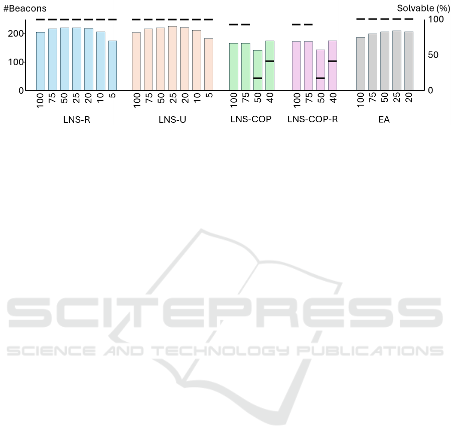
Figure 5: A visual comparison of the success probability of the different approaches and their required number of beacons.

The inability of the LNS-COP approaches to al-

ways ﬁnd a solution, as compared to COP

100

, is at-

tributed to the division of computational time across

different ﬂoors. Each level was allocated only 1

minute to ﬁnd a solution so that ultimately some time

remains for the destroy and repair process. If any

ﬂoor fails to ﬁnd a solution within the time limit,

the entire problem remains unsolved. In contrast, the

COP

100

approach tackled the entire problem as a sin-

gle instance, beneﬁting from the full 10-minute run-

time. It is anticipated that the performance of the

LNS-COP approaches would signiﬁcantly improve

with increased computational time, enabling them to

solve a greater number of problem instances.

The most promising approach overall is LNS-

COP

100

, which delivered the best solution across all

compared methods and resolutions in 21 out of 29

cases. On the other hand, it solves only 27 out of

29 instances, indicating that this approach should be

used in parallel with a robust method capable of con-

sistently ﬁnding a solution.

The evolutionary algorithm consistently ﬁnds a

solution (solvability of 100%), unlike the constraint-

based approaches. However, the solutions produced

by this method sometimes require more beacons than

the randomized LNS approach (LNS-R) and always

require more beacons than the hybrid constraint-

randomized approach (LNS-COP-R) and the LNS

constraint-based approach (LNS-COP). Interestingly,

the algorithm tends to perform best for the largest

pixel sizes, yielding the most efﬁcient solutions in

those cases.

In conclusion, both the LNS-R and EA methods

reliably produce high-quality solutions and signiﬁ-

cantly outperform the original constraint-based ap-

proach. However, the LNS-COP

100

method emerged

as the most effective, achieving the best solution in

21 out of 29 cases. For practical applications, a par-

allel portfolio approach (R

egin and Malapert, 2018)

combining these three methods (LNS-R

, EA

100

, and

LNS-COP

100

) is recommended. This combination

ensures that a high-quality solution can always be

found.

6 CONCLUSION AND FUTURE

WORK

In this work, we investigated various approaches

to solving the beacon placement problem in three-

dimensional spaces. These included a pure constraint-

based approach (COP), a randomized LNS method

with (LNS-U) and without (LNS-R) uniform ini-

tial beacon placement, two constraint-based LNS

approaches with either random (LNS-COP-R) or

constraint-based continuation (LNS-COP) for further

solution exploration, and an evolutionary algorithm

(EA). All newly developed methods signiﬁcantly

outperformed the original pure constraint-based ap-

proach, thereby enabling the practical application

of these techniques to real-world, multi-level, large-

scale buildings.

Among the proposed methods, the constraint-

based LNS approach appears particularly promis-

ing, as it often delivers high-quality solutions. Fu-

ture work will focus on advancing all the methods

presented here. Speciﬁcally, the development of

problem-speciﬁc search strategies for the constraint-

based LNS approaches seems especially promising.

As demonstrated in other problem domains (L

ofﬂer

et al., 2024), such strategies can often expedite the

discovery of an initial solution. Additionally, integrat-

ing the constraint-based LNS with local search tech-

niques, as outlined in (L

ofﬂer and Hofstedt, 2024),

holds great potential. Such an integration would al-

low leveraging the solutions from other methods (e.g.,

LNS, EA) as starting points for the constraint-based

LNS, potentially enhancing both efﬁciency and solu-

tion quality.

Solving the Three-Dimensional Beacon Placement Problem Using Constraint-Based Methods, Large Neighborhood Search, and

Evolutionary Algorithms

115

REFERENCES

Apt, K. (2003a). Constraint satisfaction problems: exam-

ples. In (Apt, 2003b). Chapter 2.

Apt, K. (2003b). Principles of Constraint Programming.

Cambridge University Press, New York, NY, USA.

Bembenik, R. and Falcman, K. (2020). BLE indoor po-

sitioning system using rssi-based trilateration. J.

Wirel. Mob. Networks Ubiquitous Comput. Depend-

able Appl., 11(3):50–69.

Christian Schulte, Mikael Lagerkvist, G. T. (2019). Gecode

6.2.0, 2019, https://www.gecode.org/, last visited

2019-11-22.

Darwin, C. (1859). On the Origin of Species by Means of

Natural Selection. Murray, London. or the Preserva-

tion of Favored Races in the Struggle for Life.

Dechter, R. (2003a). Constraint networks. In (Dechter,

2003b), chapter 2, pages 25–49.

Dechter, R. (2003b). Constraint processing. Elsevier Mor-

gan Kaufmann, San Francisco, CA 94104-3205, USA.

Demassey, S. and Beldiceanu, N. (2024). Global Constraint

Catalog. http://sofdem.github.io/gccat/. last visited

2025-05-27.

Li, G., Geng, E., Ye, Z., Xu, Y., Lin, J., and Pang, Y. (2018).

Indoor positioning algorithm based on the improved

rssi distance model. Sensors, 18:2820.

ofﬂer, S., Becker, I., B

uckert, C., and Hofstedt, P. (2023).

Enhanced optimal beacon placement for indoor posi-

tioning: A set variable based constraint programming

approach. In Gini, G., Nijmeijer, H., and Filev, D. P.,

editors, Proceedings of the 20th International Con-

ference on Informatics in Control, Automation and

Robotics, ICINCO 2023, Rome, Italy, November 13-

15, 2023, Volume 1, pages 70–79. SCITEPRESS.

ofﬂer, S., Becker, I., and Hofstedt, P. (2024). Enhancing

constraint optimization problems with greedy search

and clustering: A focus on the traveling salesman

problem. In Rocha, A. P., Steels, L., and van den

Herik, H. J., editors, Proceedings of the 16th Inter-

national Conference on Agents and Artiﬁcial Intelli-

gence, ICAART 2024, Volume 3, Rome, Italy, Febru-

ary 24-26, 2024, pages 1170–1178. SCITEPRESS.

ofﬂer, S. and Hofstedt, P. (2024). A constraint-based

greedy-local-global search for the warehouse location

problem. In Maglogiannis, I., Iliadis, L. S., MacIn-

tyre, J., Avlonitis, M., and Papaleonidas, A., editors,

Artiﬁcial Intelligence Applications and Innovations -

20th IFIP WG 12.5 International Conference, AIAI

2024, Corfu, Greece, June 27-30, 2024, Proceedings,

Part III, volume 713 of IFIP Advances in Informa-

tion and Communication Technology, pages 291–304.

Springer.

ofﬂer, S., Kroll, F., Becker, I., and Hofstedt, P. (2022). Op-

timal beacon placement for indoor positioning using

constraint programming. In 19th IEEE/ACS Interna-

tional Conference on Computer Systems and Applica-

tions, AICCSA 2022, December 5-8, 2022, pages 1–8,

Abu Dhabi, United Arab Emirates. IEEE.

Marriott, K. (1998). Programming with Constraints - An

Introduction. MIT Press, Cambridge.

McGuire, J., Law, Y. W., Chahl, J., and Do

ganc¸ay,

K. (2021). Optimal beacon placement for self-

localization using three beacon bearings. Symmetry,

13(1).

Perron, L. and Furnon, V. (2023). Google

LLC, Google OR-Tools, 2023.

https://developers.google.com/optimization/, last

visited 2025-06-11.

Popyack, J. L. (2016). Gusz eiben and jim smith (eds): In-

troduction to evolutionary computing - springer, 2015,

299 pp, ISBN: 978-3-662-44874-8. Genet. Program.

Evolvable Mach., 17(2):197–199.

Prud’homme, C. and Fages, J. (2022). Choco-solver: A java

library for constraint programming. J. Open Source

Softw., 7(78):4708.

Rajagopal, N., Chayapathy, S., Sinopoli, B., and Rowe, A.

(2016). Beacon placement for range-based indoor lo-

calization. In 2016 International Conference on In-

door Positioning and Indoor Navigation (IPIN), pages

1–8.

egin, J. and Malapert, A. (2018). Parallel constraint pro-

gramming. In Hamadi, Y. and Sais, L., editors, Hand-

book of Parallel Constraint Reasoning, pages 337–

379. Springer.

Rossi, F., Beek, P. v., and Walsh, T. (2006). Handbook of

Constraint Programming. Elsevier, Amsterdam, First

edition.

Sakpere, W., Oshin, M. A., and Mlitwa, N. B. (2017). A

state-of-the-art survey of indoor positioning and navi-

gation systems and technologies. South Afr. Comput.

J., 29(3).

Shanthi, D. L. and Chethan, N. (2023). Genetic algorithm

based hyper-parameter tuning to improve the perfor-

mance of machine learning models. SN Comput. Sci.,

4(2):119.

Sharma, R. and Badarla, V. (2018). Geometrical optimiza-

tion of a novel beacon placement strategy for 3d in-

door localization. In 2018 IEEE International Confer-

ence on Advanced Networks and Telecommunications

Systems (ANTS), pages 1–6.

Shaw, P. (1998). Using constraint programming and local

search methods to solve vehicle routing problems. In

Maher, M. and Puget, J.-F., editors, Principles and

Practice of Constraint Programming — CP98, pages

417–431, Berlin, Heidelberg. Springer Berlin Heidel-

berg.

Slowik, A. and Kwasnicka, H. (2020). Evolutionary algo-

rithms and their applications to engineering problems.

Neural Comput. Appl., 32(16):12363–12379.

van Hoeve, W.-J. and Katriel, I. (2006). Global Constraints.

In (Rossi et al., 2006), First edition. Chapter 6.

Wang, H., Rajagopal, N., Rowe, A., Sinopoli, B., and

Gao, J. (2019). Efﬁcient beacon placement algorithms

for time-of-ﬂight indoor localization. In Proceedings

of the 27th ACM SIGSPATIAL International Confer-

ence on Advances in Geographic Information Sys-

tems, Chicago, IL, USA, November 5-8, pages 119–

128.

ICINCO 2025 - 22nd International Conference on Informatics in Control, Automation and Robotics

116