Towards Machine Learning Driven Virtual Sensors for Smart Water

Infrastructure

Vineeth Maruvada

, Karamjit Kaur

, Matt Selway

and Markus Stumptner

Industrial AI, University of South Australia, Adelaide, Australia

Keywords:

Virtual Sensors, Digital Twins, Water Infrastructure, Artiﬁcial Intelligence, Machine Learning, Deep

Learning, Long Short Term Memory, XGBoost, Generative Adversarial Networks, Industry 4.0, Water

Utilities.

Abstract:

Water utilities around the world are under increasing pressure from climate change, urban expansion, and ag-

ing infrastructure. To address these challenges, smarter and more sustainable water management solutions are

essential. This study explores the use of Machine Learning (ML) to develop Virtual Sensors for smart water

infrastructure. Virtual Sensors can complement or replace physical sensors while improving environmental

sustainability and enabling reliable and cost-effective Digital Twins (DTs). Our experimental results show

that several ML models outperform traditional methods such as Auto-Regressive Integrated Moving Average

(ARIMA) in terms of forecast accuracy and timeliness. Among these, Extreme Gradient Boosting (XGBoost)

and Long Short-Term Memory (LSTM) offer the best balance between accuracy and robustness. This research

provides preliminary evidence that ML models can enable Virtual Sensors capable of delivering short-term

forecasts. When successfully implemented, Virtual Sensors can transform water utilities by improving envi-

ronmental sustainability, operational intelligence, adaptability, and resilience within Digital Twins.

1 INTRODUCTION

Water is essential for public health, economic devel-

opment, and long-term sustainability of cities. How-

ever, modern water utilities face mounting challenges

including climate change, rapid population growth,

and aging asset infrastructure, resulting in more fre-

quent asset failures, leaks, bursts, and network over-

ﬂows. This requires an intelligent and proactive ap-

proach to water management (Arnell et al., 2019).

To address these challenges, utilities need to imple-

ment smarter water infrastructure systems that en-

able early leak detection, accurate demand forecast-

ing, and predictive maintenance to minimize service

interruptions.

Physical sensors play an important role as they

generate data to efﬁciently operate water networks.

When these data are integrated with Digital Twin

(DT), these sensors form the foundation of smart wa-

ter management, allowing real-time monitoring, sim-

https://orcid.org/0000-0001-6644-8834

https://orcid.org/0000-0003-0255-1060

https://orcid.org/0000-0001-6220-6352

https://orcid.org/0000-0002-7125-3289

ulation of dynamic scenarios, and data-driven deci-

sion making (Zekri et al., 2022). However, deploying

and maintaining a dense network of physical sensors

can be prohibitively expensive and technically chal-

lenging, especially when the infrastructure is remote

or distributed. Sensor failures and data loss can dis-

rupt network and DT performance, compromising the

utility’s ability to effectively model and manage water

resources.

Artiﬁcial Intelligence (AI), and speciﬁcally Ma-

chine Learning (ML) and Deep Learning (DL), offers

a promising solution to mitigate sensor-related disrup-

tions. By learning patterns from historical data, these

models can estimate missing or faulty sensor read-

ings, effectively functioning as virtual or soft sensors

(Ibrahim et al., 2020). These virtual sensors ensure

data continuity when physical sensors fail or provide

unreliable readings, thus enhancing the resilience and

operational reliability of DT systems. Although pre-

vious studies have explored various approaches to de-

velop virtual sensors, there is still a need for system-

atic evaluation of ML methods for the water indus-

try under real-world operational conditions (Martin

et al., 2021). This study aims to ﬁll this gap by bench-

marking multiple ML models with statistical methods

Maruvada, V., Kaur, K., Selway, M. and Stumptner, M.

Towards Machine Learning Driven Virtual Sensors for Smart Water Infrastructure.

DOI: 10.5220/0013721200003982

Paper published under CC license (CC BY-NC-ND 4.0)

In Proceedings of the 22nd International Conference on Informatics in Control, Automation and Robotics (ICINCO 2025) - Volume 1, pages 453-460

ISBN: 978-989-758-770-2; ISSN: 2184-2809

453

to assess their accuracy in replicating physical sensor

measurements.

We evaluated the performance of ML models such

as XGBoost, LSTM, TadGAN, TSGAN, known for

their strong predictive capabilities, and compared

them with traditional statistical approaches such as

ARIMA. The objective is to assess whether these

models can accurately estimate sensor values when

physical readings are missing, incomplete, or noisy.

Preliminary experiments were conducted using both

single-step and multi-step time series forecasting

methods. The multi-step results exhibited reduced

predictive performance over extended horizons which

is consistent recent research highlighting error accu-

mulation in ML-based forecasting models (Marcjasz

et al., 2023). Given their limited reliability and scope,

multi-step results are not included in this study.

The structure of this paper is as follows: Section 2

reviews Virtual Sensor approaches and research gaps;

Section 3 details the Methodology; Section 4 presents

Results and Analysis; Section 5 discusses conclusion

and future work. To begin, we provide an overview

of existing literature to contextualize the development

and application of Virtual Sensors and identify key

gaps that motivate this study.

2 LITERATURE REVIEW

The following literature review covers the concept of

Virtual Sensors, their taxonomy, and concludes by

identifying research gaps.

2.1 Virtual Sensors

Virtual Sensors are models that estimate variables that

are hard or expensive to measure directly (Kadlec

et al., 2009). This approach supports the Industry 4.0

vision of adaptive and resilient systems. As shown

in Figure 1, Virtual Sensors combine physical sen-

sor data with ML output to mimic real-world sys-

tems within DTs. This enables continuous monitoring

and decision making, even when physical sensors fail,

helping to build adaptive DTs (Berglund et al., 2023;

Zahedi et al., 2024; Shen et al., 2022).

2.2 Taxonomy of Virtual Sensor Models

Based on established practices in industrial systems,

environmental monitoring, and recent developments

in DTs, virtual sensor implementations fall into the

following three broad categories:

• First-Principles Models: Based on system

physics or chemistry. Includes:

Figure 1: Virtual sensor integration in a water infrastructure

digital twin estimating missing or failed sensor values using

historical data.

– Physics-Based Models use equations based on

physical laws to model sensor behavior.

– State Observer-Based Models that estimate sys-

tem states using known dynamics

• Data-Driven Models: Rely entirely on observed

data.

– Statistical Techniques: Linear Regression, Par-

tial Least Squares (PLS), Gaussian Process Re-

gression (GPR)

– Stochastic Models: Kalman ﬁlters, Markov

models, Bayesian networks

– ML/DL Models: XGBoost, LSTM, CNN,

SVM, and GANs

• Hybrid Models:

– Physics-Informed Neural Networks (PINNs):

Embeds physical laws into neural network

training

– Other Approaches: Grey-box models, residual

learning, and combinations of physical and ML

methods.

This categorization is consistent with several key

studies in the ﬁeld (Martin et al., 2021; Weichert

et al., 2019; Psichogios and Ungar, 1992; Karni-

adakis et al., 2021; Gonz

alez-Herb

on et al., 2025),

which recognize the spectrum of approaches based on

model transparency, data availability, and computa-

tional complexity.

Earlier virtual sensor models were based on ﬁrst-

principles methods such as hydraulic equations and

state observers, which required domain expertise that

often struggled with non-linear or complex systems

(Martin et al., 2021; Weichert et al., 2019). To address

these limitations, data-driven approaches were devel-

oped. Techniques like PLS, Kalman Filters, and GPR

showed promise but they do not scale well with large

datasets (Rasmussen and Williams, 2006). Recent

advances in ML and DL, including Random Forests,

SVMs, CNNs, and LSTMs, enable modeling of non-

linear patterns and temporal dependencies (Han et al.,

ICINCO 2025 - 22nd International Conference on Informatics in Control, Automation and Robotics

454

2021; Zhao et al., 2022). Hybrid techniques are a

new and evolving area; methods like PINNs combine

physical laws with learning algorithms improve both

accuracy and interpretability. However, they may in-

troduce additional training and computational com-

plexity (Karniadakis et al., 2021). While these ad-

vances have expanded the capabilities of virtual sen-

sors, they also reveal persistent limitations that hinder

robust deployment in real-world systems.

2.3 Current Challenges and Research

Gaps

Despite advancements in physics-based and statisti-

cal modeling methods such as ARIMA, Kalman Fil-

ters, and GPR, they often struggle with the dynamic,

nonlinear, and nonstationary characteristics of real-

world water management. These models typically

lack scalability and adaptability, particularly when

dealing with high-frequency, multi-sensor data or un-

der conditions of sensor failure (Ibrahim et al., 2020;

Berglund et al., 2023). Such limitations hinder the de-

velopment of reliable DT systems, leading to subop-

timal forecasting and inefﬁcient water resource man-

agement.

To address these gaps, this study evaluates ML

models, speciﬁcally XGBoost, LSTM, and GAN vari-

ants. By benchmarking them against ARIMA, we as-

sess their ability to provide accurate forecasts. These

results align with recent research highlighting the po-

tential of ML in forecasting, anomaly detection, and

operational optimization of smart water infrastruc-

ture. Furthermore, the integration of virtual sen-

sors within IoT-enabled DT frameworks offers a scal-

able, adaptive, and cost-effective approach to monitor

the water infrastructure in real time (Lakshmikantha

et al., 2022), ultimately supporting more resilient and

intelligent water management.

3 METHODOLOGY

The following section outlines data collection from

physical sensors, the preprocessing steps, and the

modeling workﬂow. It also details the evaluation ap-

proach used to assess the performance of various ML

techniques.

3.1 Datasets and Preprocessing

This study uses two publicly available real operational

datasets collected from ﬂow sensors installed along

the Murray River. The ﬁrst dataset, from sample point

403241, captures signiﬁcant variations in ﬂow pat-

terns and includes daily measurements from 1 July

2022 to 30 June 2023. The second dataset, from sam-

ple point 403242, represents a smaller and more stable

system with daily data that span a longer period, from

1 July 2014 to 30 June 2023.

The raw datasets initially contained several at-

tributes, including Sample Point, Description, Lati-

tude, Longitude, SampleDate, Flow Category, Flow,

and Comment. To ensure consistency and relevance,

the data were preprocessed by removing non-essential

ﬁelds such as Description, Latitude, Longitude, and

Comment. Only records where the Flow Category

was set to ‘FLOW’ were retained. The datasets were

then reformatted into a standardized structure with

three key ﬁelds: SensorID, DateTime, and FlowRate.

By selecting two contrasting datasets, one with

dynamic and complex ﬂow behavior and the other

with stable operational patterns, this study helps to

provide a meaningful comparison of ML techniques

under different ﬂow scenarios. We used a univari-

ate forecasting approach that uses historical FlowRate

data as input variable.

MinMax Scaling. In univariate time-series fore-

casting, normalization of the input series is crucial

for stable and efﬁcient training. We applied Min-

Max scaling to the FlowRate series to map all histor-

ical values to a ﬁxed range, ensuring that the model

learns temporal patterns without being inﬂuenced by

the magnitude of the raw values.

MinMax scaling transforms each observed value

in the series {y

, y

, . . . , y

} to a normalized value

′

within the range [0, 1] using the following:

′

− y

min

max

− y

min

, ∀t ∈ {1, . . . , T } (1)

where y

min

= min{y

, y

, . . . , y

} and y

max

max{y

, y

, . . . , y

} represent the minimum and

maximum ﬂow values observed during training.

This operation is a linear rescaling that preserves

temporal dependencies while bounding the values to

a consistent scale.

Scaling of the data improves the numerical stabil-

ity of gradient-based models and helps mitigate issues

such as vanishing or exploding gradients. Moreover,

it ensures that lagged inputs contribute proportionally

during the learning process, allowing the model to fo-

cus on sequence patterns rather than absolute magni-

tudes (Han et al., 2011).

3.2 Feature Engineering

The main feature used for all forecasting models was

FlowRate. Although the raw data included additional

Towards Machine Learning Driven Virtual Sensors for Smart Water Infrastructure

455

attributes such as SensorID and DateTime, the focus

was on univariate forecasting, meaning that only past

FlowRate values were used as input to predict future

values. However, DateTime were used to engineer

lagged time steps and sliding windows for training the

models. These derived features were not used as in-

puts and to generate sequences of past FlowRate val-

ues to forecast the next. This approach allowed for

consistent time alignment and ensured temporal con-

tinuity across the datasets.

All models were trained using a one-step-ahead

forecasting setup, where the next FlowRate value

is predicted based on a ﬁxed window of previous

FlowRate readings. This method supports real-time

model updates and is suitable for operational scenar-

ios. Although only univariate inputs wsd used for

this study, the architecture allows future extension

to multivariate forecasting using engineered features

like day-of-week, seasonal indicators, or additional

sensor readings. Table 1 highlights the key model spe-

ciﬁc conﬁgurations used to reduce prediction errors.

3.3 Model Development

This study implements ﬁve forecasting models:

ARIMA, LSTM, XGBoost, TadGAN, and TSGAN.

The following section describes the architecture, un-

derlying algorithms, and key hyperparameter conﬁg-

urations used for each model.

3.3.1 ARIMA

The AutoRegressive Integrated Moving Average

(ARIMA) model is a classical statistical approach for

time-series forecasting. It captures linear dependen-

cies in data using a combination of autoregressive

terms, differencing operations, and moving averages.

ARIMA uses a walk-forward validation strategy, re-

training at each time step using newly available ob-

servations, making it suitable for real-time forecast-

ing scenarios, although it requires careful parameter

tuning for high-frequency or long-horizon tasks. In

this study, ARIMA is used as a statistical baseline to

evaluate the performance of more recent ML models.

Its transparent structure and interpretability provide a

valuable reference point for assessing the applicabil-

ity of data-driven approaches in the context of virtual

sensor development (Box et al., 2015).

3.3.2 XGBoost

Extreme Gradient Boosting (XGBoost) is a high-

performance ensemble learning algorithm known for

its scalability and predictive accuracy in structured

Algorithm 1: Uniﬁed forecasting procedure for ARIMA,

XGBoost, LSTM, TadGAN, and TSGAN.

Data: Preprocessed time-series y

Result: Predicted ﬂow values on the test set

Split y into training and test sets chronologically

ARIMA: begin

Initialize history and parameters (p, d, q)

For each t in test set : ﬁt model, forecast next

value ˆy

, Store ˆy

in predictions, append y

to his-

tory

end

XGBoost: begin

Generate lag, rolling, and date features

Deﬁne hyperparameter search space; Con-

duct randomized search with time-series cross-

validation

Train XGBoost regressor on training data using

selected hyper-parameters as per Table 1.

end

LSTM: begin

Create sequences with sliding window T; re-

shape as (samples, T, 1)

Deﬁne, compile and train the model with se-

lected hyper-parameters as per Table 1.

end

TadGAN: begin

Created windowed sequences; Deﬁne Generator:

LSTM Encoder-Decoder with Repeat Vector

Deﬁne Critic: Conv1D + Flatten + Dense

Compile model using selected hyper-parameters

as per Table 1.

end

TSGAN: begin

Created windowed sequences; Deﬁne Generator:

LSTM Encoder-Decoder with Dropout layers

Deﬁne Discriminator: Conv1D + Dense + Sig-

moid

Compile model using selected hyper-parameters

as per Table 1.

end

Train model and predict test values

Inverse scale predictions and test values

datasets. XGBoost operates by using sliding win-

dows of past observations to predict future values for

time series forecasting. It constructs additive regres-

sion trees through gradient boosting, allowing it to

model nonlinear dependencies. Its built-in regulariza-

tion mechanisms help mitigate overﬁtting, making it

a reliable choice for complex time-series forecasting

tasks (Chen and Guestrin, 2016).

ICINCO 2025 - 22nd International Conference on Informatics in Control, Automation and Robotics

456

Table 1: Key hyperparameter settings used for each forecasting model in this study. The settings were selected through

validation or adapted from prior work to ensure fair comparison.

Hyperparameter ARIMA XGBoost LSTM TSGAN TadGAN

Order / Estimators / Layers (2,1,2) 100 LSTM Layers - 2,

Units - 50; Dense

Layers - 20, Units - 25,

LSTM encoder (128,

64)-decoder (64,128)

LSTM encoder (100,

50)-decoder (50,100)

Learning rate — 0.1 0.001 — —

Optimizer — — Adam Adam Adam

Epochs — — 400 400 50

Batch size — — 170 170 32

Input time steps (Window size T) — — 30 30 30

Loss function MSE MSE MSE Binary Crossentropy Binary Crossentropy

3.3.3 LSTM

Long Short-Term Memory (LSTM) networks, a spe-

cialized type of recurrent neural network (RNN), are

designed to capture long-range temporal dependen-

cies and mitigate the vanishing gradient problem.

This makes them particularly effective for modeling

sequential patterns in univariate ﬂow rate data. In

our implementation, the LSTM model used a ﬁxed

input window, referred to as the timestep, to predict

the next time step’s value. This one-step-ahead fore-

casting framework ensures stable training. Multi-step

forecasting would require either recursive predictions

or a sequence-to-sequence architecture to extend the

output horizon (Hochreiter and Schmidhuber, 1997).

3.3.4 TadGAN

Time-series Anomaly Detection GAN (TadGAN) is

designed for unsupervised anomaly detection in time-

series data using a GAN architecture with an LSTM-

based generator and discriminator. It learns to re-

construct normal patterns in sequential data; anoma-

lies are identiﬁed when reconstruction errors exceed

a threshold (Geiger et al., 2020). Although, its not a

forecasting model, TadGAN can support virtual sen-

sor systems by identifying data inconsistencies or po-

tential faults in real-time monitoring streams.

3.3.5 TSGAN

Time-series GAN (TSGAN) is a generative model tai-

lored for time-series forecasting and synthetic data

generation. By learning temporal dependencies, it

produces realistic one-step-ahead predictions that can

be used to ﬁll in missing values or simulate sensor

readings (Smith and Smith, 2020). This makes TS-

GAN particularly valuable for virtual sensors, where

maintaining the continuity and plausibility of the

measurements is essential for downstream analytics

and decision-making.

3.4 Experimental Setup

All experiments were carried out within the Azure

Machine Learning Studio environment using the in-

tegrated notebook interface for code execution, data

handling, and model evaluation. Each forecasting

model was implemented in a dedicated Jupyter note-

book and organized by model type (e.g., ARIMA,

XGBoost, LSTM, GAN). These notebooks were sys-

tematically named to reﬂect the dataset version and

forecasting type, such as single-step or multi-step pre-

dictions. Data preprocessing, training, evaluation,

and visualization of results were all performed within

these notebooks to ensure reproducibility and consis-

tency between models.

Libraries and Model Conﬁguration. A

range of libraries supported model development:

statsmodels was used for ARIMA; scikit-learn

and XGBoost were used for ensemble learning; and

TensorFlow/Keras powered deep learning models

including LSTM, TadGAN, and TSGAN. Additional

packages such as pandas, NumPy, matplotlib, and

seaborn facilitated data transformation and visual-

ization. Hyperparameter tuning followed best prac-

tices, including walk-forward validation, early stop-

ping, and, where applicable, grid-based optimization

to improve generalizability and avoid overﬁtting.

Data Acquisition. Sensor data was accessed

through Azure Machine Learning Studio using a des-

ignated Azure datastore. The dataset comprised ﬂow

rate measurements tagged with DateTime and Sensor

ID. Since each model was designed to operate on data

from a single sensor, the dataset was ﬁltered accord-

ingly and sorted in chronological order to maintain

temporal integrity essential for time-series forecast-

ing.

Train-Test Splitting. The time-series data was

split into training and testing sets using an 80:20 ratio

based on temporal order. The ﬁrst 80% of the data

was used to train the models, while the remaining

20% served as the test set. This setup ensured that

only past observations were used to forecast future

values, mimicking real-world deployment scenarios.

Towards Machine Learning Driven Virtual Sensors for Smart Water Infrastructure

457

Traditional k-fold cross-validation was not employed,

as it violates the temporal sequence and risks data

leakage from future to past. Instead, the models were

trained once on the training set and evaluated on the

unseen test set. Future work may incorporate time-

series cross-validation approaches to improve evalua-

tion robustness (Bergmeir et al., 2018).

Evaluation Metrics. Model performance was

assessed using three widely accepted error metrics

(Hyndman and Koehler, 2006; Makridakis et al.,

2018): RMSE (Root Mean Squared Error), which pe-

nalizes large errors more heavily by squaring them;

MAE (Mean Absolute Error), which reﬂects the av-

erage magnitude of errors and is robust to outliers;

and R

(Coefﬁcient of Determination), which indi-

cates the proportion of variance in the observed data

explained by the model predictions.

Visual Interpretation. In addition to quantita-

tive evaluation, visual diagnostics were used to in-

terpret model performance, identify error trends, and

detect possible non-stationarity or model bias. The

forecast results were visualized using matplotlib

and seaborn, displaying training data, actual test ob-

servations and predicted values. These plots offered

an intuitive assessment of prediction accuracy across

models and time horizons. The model execution time

for the entire dataset was also recorded to provide

context on computational efﬁciency. This combina-

tion of visual and statistical evaluation ensured a com-

prehensive and transparent evaluation of the effective-

ness of the model.

4 RESULTS AND DISCUSSION

In this section, we present and interpret the results for

each model output.

4.1 Model Execution Results

Five model outputs ARIMA, XGBoost, LSTM,

TadGAN, TSGAN were compared on two real-world

datasets.

Table 2: Performance Metrics for Dataset 1 (Sensor

403241).

Model ARIMA XGBoost LSTM TadGAN TSGAN

RMSE 2245.5 1647.5 2299.5 4872.3 3068.4

MAE 1226.3 701.8 1341.3 2521.6 1468.5

0.91 0.94 0.90 0.57 0.83

Exec. Time 20sec 12sec 57sec 43sec 2min 43sec

Tables 2 and 3 present the performance of ﬁve

models applied to two real-world ﬂow sensor datasets.

XGBoost consistently achieved the highest predictive

Table 3: Performance Metrics for Dataset 2 (Sensor

403242).

Model ARIMA XGBoost LSTM TadGAN TSGAN

RMSE 3925.7 244.2 2525.2 2634.7 2162.6

MAE 1287.9 132.8 940.0 1111.3 884.6

0.86 0.99 0.91 0.90 0.93

Exec. Time 3min 9sec 14sec 4min 5sec 3min 59sec 15min 23sec

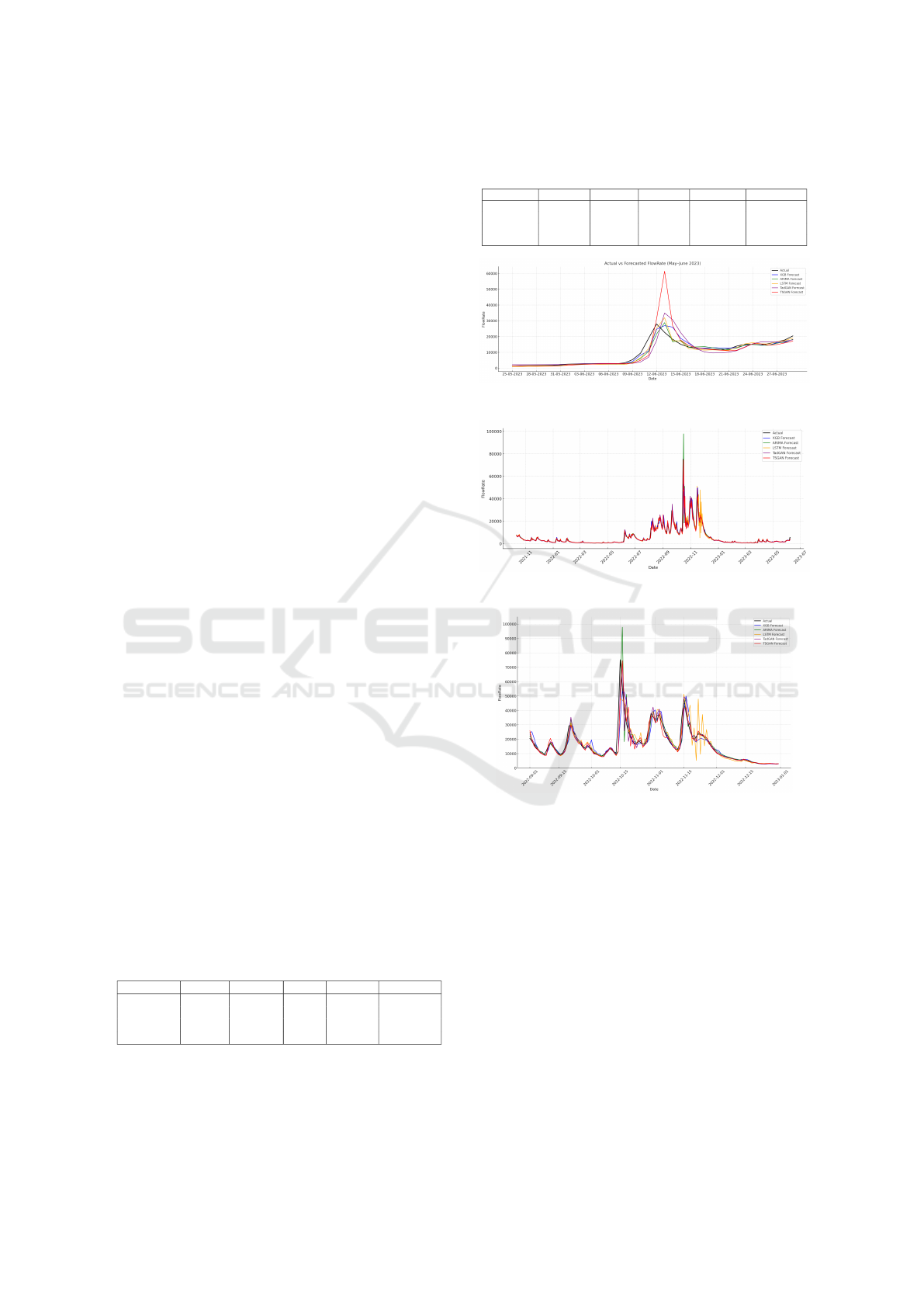
Figure 2: Results Visualization for Dataset 1.

Figure 3: Results Visualization for Dataset 2.

Figure 4: Results Visualization for Dataset 2 (Zoomed: Sep

2021–Jan 2022).

accuracy in both datasets, followed by LSTM and

TSGAN. Generative models, particularly TadGAN,

showed less stability, especially in Dataset 1, which

exhibited more variable ﬂow conditions. This initial

analysis highlights the superior performance of the

models, particularly XGBoost and LSTM, compared

to traditional statistical methods such as ARIMA.

For Sensor 403241 (Dataset 1) and Sensor 403242

(Dataset 2), XGBoost achieved the best results, with

RMSE values of 1647.5 and 244.2, and R

scores of

0.94 and 0.99, respectively. LSTM and TSGAN also

performed well, particularly in Dataset 2, where TS-

GAN demonstrated its ability to model complex, non-

linear patterns with an RMSE of 2162.6 and an R

0.93. In contrast, ARIMA showed consistently higher

ICINCO 2025 - 22nd International Conference on Informatics in Control, Automation and Robotics

458

error rates and lower explanatory power, reﬂecting its

limitations in capturing dynamic water usage behav-

iors. These ﬁndings support the growing emphasis in

the literature on the role of ML in enhancing forecast-

ing accuracy for infrastructure systems. In particular,

the model execution time for XGBoost was signiﬁ-

cantly lower compared to other models, making it a

strong candidate for real-time deployment.

Figure 2 illustrates the forecast output for Dataset

1 during the May–June 2023 period. ARIMA suc-

cessfully captured the general trend, but lagged

slightly during the peak ﬂow. XGBoost tracked the

actual data, especially during both the rising and

falling phases of the event. LSTM produced smooth

forecasts and maintained good alignment throughout,

though it slightly overestimated the peak. TadGAN

followed the ﬂow trend relatively well but over-

predicted the peak value. TSGAN exhibited the

largest overestimation at the peak, reducing its overall

accuracy in this period. Overall, XGBoost and LSTM

offered the most reliable and consistent predictions in

this scenario.

Similar patterns were observed in Dataset 2, as

shown in Figures 3 and 4. ARIMA captured the gen-

eral ﬂow trend, but struggled to respond accurately

during peak events, especially with sharp surges. XG-

Boost consistently aligned with the actual ﬂow, and

performed well across both stable and volatile peri-

ods. LSTM produced smooth forecasts overall but

exhibited increased noise and ﬂuctuations in certain

intervals, due to overﬁtting on local noise when the

training data contains high variance, combined with

its strong temporal memory. TadGAN followed the

trend reasonably but introduced ﬂuctuations around

high-ﬂow events. TSGAN demonstrated strong align-

ment with the actual values, particularly during peak

periods, and outperformed other generative models.

Overall, XGBoost and TSGAN provided the most re-

liable forecasts for Dataset 2.

4.2 Model Performance Insights

Our evaluation of models reveals that modern ML

approaches, particularly XGBoost and LSTM, con-

sistently outperformed traditional statistical methods

such as ARIMA in ﬂow prediction tasks. XGBoost

achieved the highest accuracy across both datasets,

with an RMSE of 1647.50 and R

of 0.94 in Dataset 1,

and an even stronger RMSE of 244.17 and R

of 0.99

in Dataset 2. LSTM also performed robustly, effec-

tively capturing temporal patterns. Among generative

models, TSGAN showed potential in modeling non-

linear dynamics, achieving an R

of 0.93 on Dataset

2 but struggled with irregular patterns in Dataset 1.

ARIMA, by contrast, produced consistently higher er-

rors and lower R

scores, highlighting its limitations

in dynamic systems.

While XGBoost and LSTM were generally reli-

able, their effectiveness varied by dataset, underscor-

ing the importance of tailoring virtual sensor models

to speciﬁc environments. Regular retraining based on

evolving demand is critical to ensure sustained ac-

curacy. Integrating such models within DT frame-

works would enable automated updates and support

real-time operational monitoring.

These results suggest that ML models can serve

as effective tools for immediate data imputation and

near term prediction. However, more work is needed

to extend these beneﬁts to long-term prediction sce-

narios. Overall, these insights offer practical guid-

ance for water utilities seeking to adopt ML and DL

techniques. By prioritizing robust models like XG-

Boost and LSTM, and exploring the integration of

generative approaches for anomaly detection and data

gap ﬁlling, utilities can signiﬁcantly enhance the re-

silience, scalability, and decision making capabilities

of smart water infrastructure.

5 CONCLUSION AND FUTURE

WORK

This study investigates the potential of machine

learning-based virtual sensors to replicate physical

sensor output using historical ﬂow data from two

key locations. Preliminary results show that short-

term ﬂow forecasts can be generated accurately

and efﬁciently using models such as XGBoost and

LSTM. Both models outperformed traditional statis-

tical methods such as ARIMA in terms of predictive

accuracy and computational efﬁciency. In particular,

XGBoost delivered the best balance between speed

and performance, positioning it as a practical solution

for ﬁlling data gaps and supporting short-term fore-

casts.

Although these results are based on historical data

under known conditions, they demonstrate the strong

potential of XGBoost and LSTM for developing vir-

tual sensors in water infrastructure. Future work

should focus on validating these models using real-

time water network data, integrating insights from

correlated sensors, and enhancing multi-step forecast

capabilities. With further reﬁnement, ML-based vir-

tual sensors could play a critical role in improving the

resilience, and responsiveness of smart water infras-

tructure.

Towards Machine Learning Driven Virtual Sensors for Smart Water Infrastructure

459

REFERENCES

Arnell, N. W. et al. (2019). Global and regional impacts of

climate change at different levels of global tempera-

ture increase. Global Environmental Change, 58:101–

113.

Berglund, E. Z., Shaﬁee, M. E., Xing, L., and Wen, J.

(2023). Digital twins for water distribution systems.

Journal of Water Resources Planning and Manage-

ment, 149(3):02523001.

Bergmeir, C., Hyndman, R. J., and Koo, B. (2018). A

note on the validity of cross-validation for evaluating

autoregressive time series prediction. Computational

Statistics & Data Analysis, 120:70–83.

Box, G. E. P., Jenkins, G. M., Reinsel, G. C., and Ljung,

G. M. (2015). Time Series Analysis: Forecasting and

Control. Wiley, Hoboken, NJ, 5th edition.

Chen, T. and Guestrin, C. (2016). Xgboost: A scalable

tree boosting system. In Proceedings of the 22nd

ACM SIGKDD International Conference on Knowl-

edge Discovery and Data Mining, pages 785–794.

ACM.

Geiger, A., Liu, D., Alnegheimish, S., Cuesta-Infante, A.,

and Veeramachaneni, K. (2020). Tadgan: Time series

anomaly detection using generative adversarial net-

works. In IEEE Int’l. Conf. on Big Data (Big Data

’20’), pages 33–43. IEEE.

Gonz

alez-Herb

on, R., Gonz

alez-Mateos, G., Rodr

ıguez-

Ossorio, J., Prada, M., Mor

an, A., Alonso, S., Fuertes,

J., and Dom

ınguez, M. (2025). Assessment and de-

ployment of a lstm-based virtual sensor in an indus-

trial process control loop. Neural Computing and Ap-

plications, 37(17):10507–10519.

Han, J., Kamber, M., and Pei, J. (2011). Data Mining: Con-

cepts and Techniques. Elsevier, Burlington, MA, 3rd

edition.

Han, Z., Zhao, J., Leung, H., Ma, K.-F., and Wang, W.

(2021). A review of deep learning models for time

series prediction. IEEE Sensors Journal, 21(6):7833–

7848.

Hochreiter, S. and Schmidhuber, J. (1997). Long short-term

memory. Neural Computation, 9(8):1735–1780.

Hyndman, R. J. and Koehler, A. B. (2006). Another look at

measures of forecast accuracy. International Journal

of Forecasting, 22(4):679–688.

Ibrahim, T., Omar, Y., and Maghraby, F. A. (2020). Wa-

ter demand forecasting using machine learning and

time series algorithms. In 2020 International Confer-

ence on Emerging Smart Computing and Informatics

(ESCI), pages 325–329. IEEE.

Kadlec, P., Gabrys, B., and Strandt, S. (2009). Data-driven

soft sensors in the process industry. Computers &

Chemical Engineering, 33(4):795–814.

Karniadakis, G. E. et al. (2021). Physics-informed machine

learning. Nature Reviews Physics, 3(6):422–440.

Lakshmikantha, V., Hiriyannagowda, A., Manjunath, A.,

Patted, A., Basavaiah, J., and Anthony, A. A. (2022).

Iot based smart water quality monitoring system. Ma-

terials Today: Proceedings, 51:1283–1287.

Makridakis, S., Spiliotis, E., and Assimakopoulos, V.

(2018). Statistical and machine learning forecasting

methods: Concerns and ways forward. PLoS ONE,

13(3):e0194889.

Marcjasz, G., Narajewski, M., Weron, R., and Ziel, F.

(2023). Distributional neural networks for electricity

price forecasting. Energy Economics, 125:106843.

Martin, D., K

uhl, N., and Satzger, G. (2021). Virtual sen-

sors. Business & Information Systems Engineering,

63:315–323.

Psichogios, D. and Ungar, L. (1992). A hybrid neural

network-ﬁrst principles approach to process model-

ing. AIChE Journal, 38(10):1499–1511.

Rasmussen, C. E. and Williams, C. K. I. (2006). Gaussian

Processes for Machine Learning. MIT Press.

Shen, Y. et al. (2022). Digital twins for smart water manage-

ment: Framework and case studies. Water Research,

218:118449.

Smith, K. E. and Smith, A. O. (2020). Conditional

gan for timeseries generation. arXiv preprint

arXiv:2006.16477.

Weichert, D. et al. (2019). A review of machine learning

for the optimization of production processes. Interna-

tional Journal of Advanced Manufacturing Technol-

ogy, 104(9–12):3663–3682.

Zahedi, F., Alavi, H., Majrouhi Sardroud, J., and Dang, H.

(2024). Digital twins in the sustainable construction

industry. Buildings, 14(11):3613.

Zekri, S., Jabeur, N., and Gharrad, H. (2022). Smart water

management using intelligent digital twins. Comput-

ing and Informatics, 41(1):135–153.

Zhao, Z., Chen, W., Wu, X., Chen, P., Liu, J., Chen, J.,

and Deng, S. (2022). Deep learning for time series

forecasting: A survey. Artiﬁcial Intelligence Review,

55:4099–4139.

ICINCO 2025 - 22nd International Conference on Informatics in Control, Automation and Robotics

460