Calibration Architecture for the Nonlinear Wheel Odometry Model with

Integrated Noise Compensation

e Fazekas

1,2 a

and P

eter G

asp

1 b

HUN-REN Institute for Computer Science and Control, Hungarian Research Network (HUN-REN SZTAKI),

Kende Street 13-17, Budapest, 1111, Hungary

Department of Control for Transportation and Vehicle Systems, Budapest University of Technology and Economics

(BME-KJIT), Stoczek street 2, Budapest, 1111, Hungary

Keywords:

Parameter Identiﬁcation, Wheel Odometry, Gauss-Newton, Optimal Control, Localization, Autonomous

Vehicle.

Abstract:

In the motion estimation of self-driving vehicles, the three main requirements are accuracy, robustness, and

cost-effectiveness. The generally applied sensors and methods are the GNSS, inertial, and visual-odometry, but

the contradictory requirements demand the integration of new ideas. The wheel odometry could be an adequate

choice since the method is robust and cost-effective, but the accuracy of the estimation is limited by the

parameter uncertainty, thus a calibration method should be included as well. However, the general parameter

identiﬁcation of a nonlinear model in the presence of noise has not been solved yet. The presented method is

based on the assumption that noisy, but several measurements of GNSS and IMU sensors are available in a

self-driving vehicle. In the proposed architecture, nonlinear least squares and optimal control techniques are

combined in a unique way to compensate for the noise of the orientation and wheel rotation signals to achieve

unbiased model calibration. The performance of the developed algorithm and the accuracy of parameter

estimation are demonstrated with detailed validation and a test with a real vehicle.

1 INTRODUCTION

State estimation plays a critical role in self-driving

because trajectory planning and motion control are

based on its results. The aim is to determine the

velocities and pose signals as accurately as possible.

Similarly, robustness and cost-efﬁciency are also im-

portant in the automotive industry, thus cost-effective

automotive-grade types of sensors are applied gener-

ally. The disadvantages of the GNSS (Global Navi-

gation Satellite System), IMU (inertial measurement

unit), or vision-based methods can be mitigated with

the integration of wheel encoder measurements (Funk

et al., 2017), (Sebastian Thrun, 2006). An accurate

wheel odometry model would open up new possibil-

ities to eliminate the drawbacks of the usual global

navigation-centered GNSS-inertial-visual estimation

for vehicles (Gao et al., 2018), (Falco et al., 2017), for

example, it would be possible to correct the pseudor-

ange measurements of the GNSS modules, which im-

proves the performance of the whole state estimation.

https://orcid.org/0009-0007-2157-4053

https://orcid.org/0000-0003-3388-1724

Furthermore, in GNSS-denied environments, the ne-

cessity of wheel odometry is indisputable. However,

the model suffers from parameter uncertainty. There-

fore, this paper focuses on the calibration of the wheel

odometry model, which is equivalent to the parameter

identiﬁcation of a nonlinear dynamic system. Gener-

ally, this type of optimization has not been solved yet,

see e.g. (Schoukens and Ljung, 2019), and the prob-

lem is more difﬁcult when the model calibration has

to be performed with noisy signals.

The calibration problem of the wheel odometry

model ﬁrst appeared in the navigation task of small

mobile robots and has also become a topic of investi-

gation with the appearance of autonomous functions

in the automotive industry. The related works op-

erate with two different estimation methods. In the

one, the parameter estimation is handled as a state ﬁl-

tering with the Augmented Kalman-ﬁlter (Martinelli

and Siegwart, 2006; Brunker et al., 2017). The pro-

cess assumes zero dynamics for the parameters, thus

it is a simple way to identify unknown values, but the

convergence and observability are questionable (Mar-

tinelli and Siegwart, 2006; Censi et al., 2013), and

Fazekas, M. and Gáspár, P.

Calibration Architecture for the Nonlinear Wheel Odometry Model with Integrated Noise Compensation.

DOI: 10.5220/0013720800003982

Paper published under CC license (CC BY-NC-ND 4.0)

In Proceedings of the 22nd International Conference on Informatics in Control, Automation and Robotics (ICINCO 2025) - Volume 2, pages 325-332

ISBN: 978-989-758-770-2; ISSN: 2184-2809

325

a ﬁnal stable value can not be obtained. The other

method is to estimate the parameters as a regression

problem, which, due to the nonlinear model, results in

non-convex optimization. Its general solution is difﬁ-

cult, the methods such as (Censi et al., 2013; Seeg-

miller et al., 2013) manage the nonlinear problem

with double linearization or separation, however these

only operate with a simpliﬁed odometry model and al-

most perfect reference orientation measurements. In

the case of a real-sized self-driving vehicle, these can

not be presumed (Fazekas et al., 2020).

When parameters of a nonlinear model are identi-

ﬁed, the key factor is the handling of the noise. Linear

system identiﬁcation is a well-explored area (Ljung,

1987), but due to nonlinearity, there are new issues

that do not appear at all in the linear case. Since the

dynamics from the inputs to the outputs is not linear,

the impact of the input noise can not be modeled with

Gaussian distribution (which assumption is applied in

the methods such as Kalman-ﬁltering or least squares)

on the measured output (Schoukens and Ljung, 2019).

Thus, the model calibration will certainly be biased,

even in the case of white noise.

This distortion effect can be handled in two ways.

The one is to apply speciﬁc requirements, such as un-

biased estimation of the initial pose (Antonelli et al.,

2005), measurement with expensive sensors (Lemmer

et al., 2010), or special pre-deﬁned measurement sce-

narios (Jung et al., 2016), etc. Only a few papers use

the other way, which is to develop a unique algorithm

that deals with the noise. In (Maye et al., 2016), an

undesirable behavior of the traditional observability

analysis is examined. The proposed algorithm detects

the case when, due to the noise, the parameters seem

to be observable, but in fact, they are not (e.g. the ve-

hicle moves on a degenerate path for the calibration).

In parallel with the machine learning boom, stud-

ies apply machine learning techniques to the odom-

etry calibration topic. In (Onyekpe et al., 2021), a

neural network is trained to learn the pose error of a

mobile robot, and an improved version in (He et al.,

2023) for real-sized vehicles, but the online recalibra-

tion is not addressed. Other works, such as (Toledo

et al., 2018) and (Zhang et al., 2021), approximate the

whole odometry model instead of the error. Regard-

less of whether the error or the model is learned, spe-

cial attention should be taken to avoid overﬁtting, as

the training data’s actual measurement error includes

the noise and it is also approximated. Another dis-

advantage is that the industry prefers physical mod-

els to black-box models, especially for safety-critical

systems such as automated road vehicles. Therefore,

these can be rather a supplementary method and more

important is the detailed physical modeling and the

calibration of its parameters, before the approxima-

tion of the remaining error terms.

Our work addresses the direct compensation of

the distortion effect of the noise. Any speciﬁc re-

quirement is not applied, since a self-driving vehi-

cle should recalibrate itself with the available onboard

sensors. Only measurements of general driving in real

streets are used, without any predeﬁned path or in-

put sequence. The main contribution is that the pro-

posed calibration architecture includes noise compen-

sation besides the traditional parameter identiﬁcation.

The algorithm operates with the Gauss-Newton non-

linear least squares method and an optimal control

technique. The efﬁciency of the proposed algorithm

is validated with experimental tests of a real-sized ve-

hicle, which demonstrates that the mentioned issues

of the noise are eliminated, and unbiased model cali-

bration can be reached.

The remainder of the paper is organized as fol-

lows. In Section 2, the applied odometry model, in-

cluding a dynamic wheel model, is presented. The

general calibration method of a nonlinear model is

described in Section 3. This section also outlines the

problems and gives a brief review with motivation ex-

amples. The proposed improved calibration architec-

ture with noise compensation can be found in Section

4. The validity of our approach is demonstrated via

vehicle test experiments and detailed tests in Section

5, and ﬁnally, the paper is concluded in Section 6.

2 VEHICLE MODEL

The navigation with wheel odometry is based on a

model, where the state vector x

contains the pose,

the longitudinal and lateral positions of the center of

gravity p

x,t

, p

y,t

, and the ψ

orientation of the vehicle,

and change of the pose is based on the longitudinal

t−1

and angular ω

t−1

velocities,





x,t

y,t









x,t−1

+ v

t−1

· cos(ψ

t−1

+ β

t−1

)

y,t−1

+ v

t−1

· sin(ψ

t−1

+ β

t−1

)

t−1

+ ω

t−1





(1)

The input u

is composed of the n

l,t

effective

wheel rotation signals (l = RL, RR rear-left/right),

which are the slip free rotations, and the β

sideslip

angle of the vehicle.

The velocities are computed utilizing the wheel

rotations,

= (n

RL,t

· c

RL,t

+ n

RR,t

· c

RR,t

)/2, (2a)

= (n

RR,t

· c

RR,t

− n

RL,t

· c

RL,t

)/t

, (2b)

ICINCO 2025 - 22nd International Conference on Informatics in Control, Automation and Robotics

326

Figure 1: Odometry model.

where c

l,t

is the actual wheel circumference, and t

is the rear track. The slight change of the wheel ra-

dius due to the effect of vertical dynamics is generally

neglected, because the odometry-based localization is

widely used in low-speed circumstances, e.g. auto-

mated parking. However, our method is developed

for general driving, where the dynamics is signiﬁcant,

thus we apply the proposed model of (Fazekas et al.,

2020), in which the change is considered, such as

RL,t

= c

+ c

/2 + d · a

y,t

, (3a)

RR,t

= c

− c

/2 − d · a

y,t

, (3b)

where the c

is the effective wheel circumference, c

is the difference between the effective values, a

y,t

the lateral acceleration, and the dynamic component

d takes into account the effect of vertical dynamics.

In the calibration process, every state variable is mea-

sured, thus the system model is

= f (x

t−1

,θ), x

= [p

x,t

, p

y,t

,ψ

]

, (4a)

= [n

RL,t

RR,t

,β

y,t

]

, y

= x

, (4b)

and the vehicle model parameters are arranged in the

parameter vector,

θ = [c

,d]. (5)

The values are illustrated in the paper with the

units of m,mm,m,mm·s

/m for the c

,d parame-

ters, respectively. The nominal values of c

and t

can

be found in the vehicle datasheet, but with these val-

ues, the position error of the model is already in the

range of 10 m after a few hundred meters.

3 CALIBRATION OF

NONLINEAR MODELS AND

MOTIVATION EXAMPLES

3.1 Parameter Estimation with

Gauss-Newton Method

Generally, the parameter estimation is formulated as a

least squares (LS) optimization problem, to minimize

the error of the

(θ) predictor of the model from

output measurements, such as

opt

= arg min

(θ) = arg min

∑

k=1

−

(θ)||

(6)

When the model is nonlinear in θ the optimization

can only be solved with numerical search (Tangirala,

2015). We apply the Gauss-Newton (G-N) method

that solves the nonlinear least squares problem with

Taylor-approximation in the following way,

(θ) ≈

(θ

i−1

) +

∂

(θ)

∂θ



i−1

| {z }

(θ − θ

i−1

)

| {z }

∆θ

. (7)

Due to the dynamic behavior of the predictor, the

jacobians are computed recursively. This results in

a locally linear LS problem, such as

∆θ

opt

= arg min

∆θ

∑

k=1

||(

−

(

i−1

)) − j

∆θ||

, (8)

which can be solved with the LS solution in an itera-

tive way,

i−1

+ (J

W J)

−1

W R, (9)

where the J := J(

i−1

), R :=

Y −

Y (

i−1

) matrices are

formed from the j

and (

−

(

i−1

) values, respec-

tively. A weight matrix W is also added to the basic

solution. Since the model is linearized in the previ-

ous parameters, an initial guess for θ is required, and

when in last term (

Y −

Y (

i−1

)) the integrated system

model is computed, the states have to be initialized at

the beginning of the estimation window.

3.2 Problems of Nonlinear Parameter

Estimation

The noise on the

measured output would be less sig-

niﬁcant because it enters after the nonlinearity. How-

ever, when the R residual in (9) is formulated, the

t→k=0

measured output has to be utilized for state

initialization. Due to the appeared noise on it, the in-

tegrated model diverges from the correct path regard-

less of the vehicle parameters, which results in bias in

the model calibration. Some paper tries to deal with

the issue (Fazekas et al., 2021b), but the general solu-

tion is still an open question.

The noise on the u

measured input must not be ne-

glected, since its impact on the output can not be mod-

eled with the Gaussian framework (Schoukens and

Ljung, 2019). Because the methods like least squares

or Kalman-ﬁlter apply this framework, the estimation

would be biased. Therefore, our paper focuses on the

compensation of both input and output noises to guar-

antee unbiased model calibration.

Calibration Architecture for the Nonlinear Wheel Odometry Model with Integrated Noise Compensation

327

3.3 Motivation Examples of the

Calibration and Compensation

Without calibration of the odometry model, c

=0 and

d=0, and nominal values as c

=2 m, and t

=1.55 m

have to be utilized. The localization error with this

setting is 6 m on 150 m long segments, thus the model

without calibration is useless for vehicle localization.

The amount of distortion due to uncertain pa-

rameters and wheel rotation input noises, simulated

signals are generated where the measured (n

RL/RR

)

wheel rotation signals are ﬁltered with a Fourier-

transformation, and these are utilized as inputs in the

odometry model (4a) to form noise-free signals.

3.3.1 Impact of the Parameter Uncertainty and

Initialization

The positioning uncertainty is almost linear with the

parameter uncertainty. The circumference difference

has the highest impact, the deviation of around 2 mm

of c

has the same 2 m mean position error as 2.5

cm of c

, 5 cm of t

, or 2 mm · s

/m of d parameter

uncertainty.

The noisy measurements used for state initial-

ization (x

k=0

) result in similar path divergence

in the integrated model. For example, calibrating

the model with additive Gaussian pose noises with

= σ

= 0.2 m, and σ

= 1.5

◦

standard deviation,

the bias of the estimated parameters are 7.82e-04 m,

0.24 mm, 0.09 m, 1.26 mm for the c

,d param-

eters, respectively. The consequence of these uncer-

tain calibrations is a 2.26 m validation error on 150

m long routes. The noise on the orientation initializa-

tion is mainly responsible for the error, thus for proper

odometry calibration, the measured orientation has to

be corrected.

3.3.2 Impact of the Wheel Rotation Noise

For the examination of the impact of wheel rota-

tion noise, generated Gaussian noise signals with

n,RL/RR

= 0.0005 (at 50 km/h the n

RL/RR,t

signals are

0.17 due to the multiplication by the sampling time)

are added to the ﬁltered signals. Since the simulated

pose signals are utilized for the calibration, the de-

viation from the noise-free case is induced only by

the noise of the wheel rotation. The biases of the

identiﬁed parameters are 0.0002 m, 0.31 mm, 0.25

m, 0.7 mm for the c

,d parameters, respectively,

but the middle 50% IQR ranges of the estimated val-

ues are spread within the 0.003 m, 1.2 mm, 0.1 m,

2.2 mm ranges. Previous examinations illustrate that

these deviations result in signiﬁcantly increased posi-

tion error, which can be found in Figure 2. The 1 m

Figure 2: Mean position errors with σ

n,RL/RR

= 0.0005 ad-

ditive wheel rotation noise.

position error demonstrates the necessity of compen-

sating the wheel rotation signals as well, since even

with this generated noise with zero mean, the result-

ing localization inaccuracy is signiﬁcant.

4 CALIBRATION METHOD

WITH INTEGRATED NOISE

COMPENSATION

4.1 Estimation in Batch Mode

The mentioned problems in Section 3.2 can be han-

dled if more K long measurement segments are ap-

plied at once. In this batch mode, the matrices in the

G-N method of the segments are concatenated into the

following huge matrices (N denotes the batch size),

(

i−1

) =







(

i−1

)

(

i−1

)













−

(

i−1

)

−

(

i−1

)







(10)

The parameters can be identiﬁed in the same iterative

way of (9) with the batch matrices, as

B,i

B,i−1

+ (J

)

−1

, (11)

In this case, the model ﬁtting is performed on ev-

ery segment simultaneously, which reduces the effect

of noise. However, the distortion effect of the noises

is only reduced but not eliminated, since the segment

with the highest residual has a higher impact on the re-

sulting common estimated parameters due to the min-

imization of the sum of residuals.

4.2 Input Compensation Method

The main inputs of the odometry model to be com-

pensated are the effective wheel rotations, which will

be noted as u

c,t

= [n

RL,t

RR,t

]

. These are measured

with the ABS encoder, but the quantities are corrupted

by the slip and measurement noises.

For the compensation of the wheel rotation input

noises, a minimization task is formed such as,

min

(·)

∑

k=1



(θ),u

c,k



s.t. x

= f (x

k−1

,θ) | x

(12)

ICINCO 2025 - 22nd International Conference on Informatics in Control, Automation and Robotics

328

which is the general optimal control problem in dis-

crete form (y

(θ) = x

the model output). The idea is

motivated by the well-known model predictive con-

trol strategy, where the optimal input sequence can be

determined with numerical optimization to satisfy the

tracking of a future trajectory by the system.

In the nonlinear case, it is meaningful to apply

quadratic cost functions and perform Jacobian lin-

earization of the model around a nominal trajectory,

∂ f (·)

∂x



∂ f (·)

∂u



, (13a)

= f (

k−1

,θ)− (A

k−1

+ B

k−1

). (13b)

With these considerations, the optimization prob-

lem (12) can be traced back to a locally linear predic-

tive control minimization with equality constraints.

The following task can be solved with quadratic pro-

gramming (QP) techniques,

min

(·)

∑

k=1

− y

(θ)||

+ ||∆u

c,k

→ ˘u

(·)

s.t. x

k−1

| x

≤ x

, u

c,k

≤ u

c,k

≤ u

c,k

k = 1...K

(14)

where Q, and R are positive deﬁnite weighting ma-

trices. The nominal trajectory

k=1..K

is computed

with the model (4a) utilizing the measured

c,k=1..K

wheel rotations. The QP solvers apply initial values

for the optimization to which the measured values are

applied as well.

4.3 Calibration Architecture

Our method operates with automotive-grade dual

GNSS, IMU and wheel encoder sensors. The details

of the measurements can be found in Section 5.1, now,

assume to have measured pose (

ψ), wheel ro-

tation (

), and the required additional inputs of

the model (β, a

The aim of this paper is the proper model calibra-

tion through noise compensation. However, the opti-

mal control task (12) supposes a known θ parameter,

and correct pose values are required for the state ini-

tialization. Therefore, a complex architecture is pro-

posed, which can be found in Figure 3. The algorithm

operates with smaller segments divided from a long

measurement, and it has the following 5 steps:

Step 1: Prior parameter estimation

To generate parameters for the input estimation, ini-

tial G-N identiﬁcations are performed in batch mode

(Section 4.1) resulting

values.

Step 2: Orientation correction

Figure 3: Architecture of the model calibration. In every

step, the actual version of the utilized input and output sig-

nals are illustrated.

The wheel rotation compensation method presented

in Section 4.2 is applicable for the orientation correc-

tion as well. As a result of the minimization, besides

the optimal inputs, the states are also estimated. To

minimize the trajectory error in (14), the evolution of

estimated wheel rotation signals in the initial time in-

stants generates a signiﬁcant change in the orienta-

tion, which is equivalent to the compensation of the

initialization error. The compensated orientation is

formulated as,

+ ∆ψ, ∆ψ = (

(

, ˘u

) −

), (15)

where

(θ

, ˘u

) is the orientation value with the es-

timated optimal inputs at the k = 10 time moment.

This compensation is performed for every segment of

the batch individually.

Step 3: Compensated parameter estimation

Since the orientation signal of the segments is com-

pensated, the same batch parameter estimation as in

Step 1 is recalculated. In this way,

initial param-

eters with increased accuracy are formulated for the

input estimation.

Step 4: Rotation input estimation

The wheel rotation compensation is performed with

the optimal control algorithm. The estimated

val-

ues are utilized, and the vehicle model is parameter-

ized with

. Since more

values are available, the

input estimation is performed more times, and com-

pensated

RL/RR

signals are formed as the mean of the

middle 80% of ˘u

estimations.

Step 5: Final parameter estimation

Finally, the vehicle parameters are identiﬁed in batch

mode resulting in the

identiﬁed values, but at this

time in every segment, the compensated

and

inputs, and

orientation are utilized.

Calibration Architecture for the Nonlinear Wheel Odometry Model with Integrated Noise Compensation

329

4.4 Tuning of the Method Through an

Illustration Example

In the Gauss-Newton parameter identiﬁcation

method, the W is introduced to equalize the lower

value of orientation error in radians, than the position

errors in meters. The experimental tuning results in

the following setting

w = [w

] = [1,1,50], W = [w,...,w]

1×3K

to obtain proper vehicle model calibration. Due to

the linearization in the G-N method, an initial guess

for the parameters is necessary, for which the nomi-

nal values as θ

nom

= [2,0,1.55, 0] from the vehicle’s

datasheet are applied. The maximum iteration of the

G-N method is 5.

Since in our optimal control problem the esti-

mated inputs are measured and close to the effective

ones, a relatively high prediction horizon K = 650 can

be applied. For maximum iteration, 10 is sufﬁcient,

due to the limits being chosen such as,

− [5,5,0.5], x

+ [5,5,0.5],

c,k

· 0.95, u

c,k

· 1.05.

The main tuning parameters of the optimal con-

trol task are the Q and R weighting matrices as Q =

diag([q

]) and R = diag([r

]). En-

suring the trajectory tracking without high-frequency

changes of inputs, the weights are chosen, such as

= 1, q

= 1, r

= 1000, r

= 1000,

= 1 in Step 2, q

= 10 in Step 4.

The batch size of the G-N method and the num-

ber of input estimations to form the compensated sig-

nals inﬂuence the accuracy of model calibration. The

batch size is ﬁxed through the algorithm to N = 9,

and when the

RL/RR

signals are estimated, 12 input

estimations are performed.

5 RESULTS

5.1 Test Vehicle and Measurement

The test vehicle is equipped with automotive-grade

GNSS, compass, and IMU sensors, and from the ve-

hicle’s CAN bus, the wheel encoder signals are also

saved with 0.025 s sampling time. The test track is a

24 km long route in suburban and city driving, con-

taining various bends, two roundabouts, and lots of

crossroads.

The signals of the GNSS, compass, and IMU sen-

sor are utilized in a Kalman-ﬁlter (Caron et al., 2006)

to compute the measured

ψ pose values. The

sideslip is also estimated with an IMU-based method

(Fazekas et al., 2021a) in the bends.

The calibration architecture operates with smaller

measurement parts, therefore, the route is divided into

segments with 150 m average length. Since the c

and d parameters can be appropriately observed only

with the yaw rate equations (2b), the 896 segments

with absolute angular velocity higher than 0.15 rad/s

are selected for the parameter estimation. Using these

segments, 1000 various batches are formulated.

5.2 Validation Process and Error

The true value of the θ = [c

,d] parameters are

unknown, thus the presented method is validated with

the position error of the calibrated models. In order to

avoid overﬁtting, the segments are regenerated with

300 m average length for the validation. The position

error of a calibration containing

θ is calculated for ev-

ery segment s,

p,s

∑

k=1

(

x,k

− p

x,k

(

θ))

+ (

y,k

− p

y,k

(

θ))

(16)

and the E

= E

p.s

average of these is applied as a val-

idation error to evaluate the calibration.

The minimum validation error is not zero, because

the states of the odometry model (4a) at the beginning

are initialized with the

measured pose values, and

raw

RL/RR,t

rotations are utilized. The reachable limit

in this validation case is 2.42 m, and the calibrations

are presented compared to this value.

5.3 Prior Model Calibrations

To reach initial estimated parameters, the batch G-

N method (Section 4.1) is utilized on the formulated

1000 batches. In Step 1, the raw measured

pose and

RL/RR,t

rotations are utilized. The estimated parame-

ters can be found in Figure 5, the standard deviations

of the quantities are high, e.g. the track width reaches

both 1.45 m and 1.65 m, which are unrealistic. The

top boxplot of Figure 6 shows the validation error, the

median value is 0.8 m, but due to the uncertain pa-

rameters, the error reaches 3.5 m.

5.4 Orientation Compensation and

Illustration of the Input Estimation

It has been mentioned that an interesting property of

the input estimation is the capability of correcting the

orientation measurement uncertainty as well. For a

ICINCO 2025 - 22nd International Conference on Informatics in Control, Automation and Robotics

330

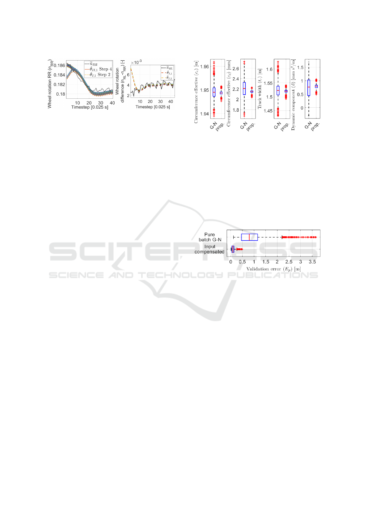
Figure 4: Estimated wheel rotation signals of a segment.

segment, the orientation correction (Step 2) is per-

formed with more θ

prior parameters. The left of

Figure 4 presents a part of the estimated wheel rota-

tions. The estimated signals are close to each other

with a similar shape. In the case of orientation cor-

rection, the difference of the rotations is worth exam-

ining in the right of Figure 4.

Initially, the difference between the estimated sig-

nals is signiﬁcantly greater than the difference be-

tween the measured rotations, indicating a determin-

istic occurrence. The change of the wheel rotation dif-

ference induces additional angular velocity, thus the

orientation can be compensated via the input estima-

tion method.

The estimated orientation difference (∆ψ) of all of

the segments in the batches is in the range of ±3

◦

with

IQR of [-0.7

◦

,0.6

◦

], which has a signiﬁcant impact on

the estimations, therefore the orientation compensa-

tion is absolutely necessary.

In Step 4, the same input estimation is executed

with the segments as in Step 2, but the

ψ estimated

orientation is utilized. The left of Figure 4 shows that

the fall at the beginning disappeared owing to the im-

proved initialization, and the estimated rotations are

around the measured ones. However, the plot illus-

trates that the optimized trajectory tracking induces

smoother wheel rotations and veriﬁes the assumption

of noisy measured signals. The variety of the estima-

tions is ﬁltered out with the formulation of the mean

of the ˘u

signals to reach

RL/RR

5.5 Calibration with the Proposed

Method and Validation

Finally, in Step 5, the vehicle parameters are esti-

mated in batch mode utilizing the estimated

ψ and

RL/RR

signals. For comparison, the same batches are

used as in Step 1. The process illustrated in Figure 3

is performed for every batch. The estimated parame-

ters of the 1000 batches are shown with box-plots in

Figure 5. The medians of the identiﬁed parameters

are almost the same as in Step 1 with the pure batch

G-N, but the standard deviations of the calibrations

decrease substantially.

Figure 5: Box-plots of the estimated parameters with the

pure (Step 1) and proposed (Step 5.) method.

The ranges of the middle 50% of the parameters

are decreased by 78%, 87%, 80% and 84%, of the c

, t

, d parameters, while the spreads of estimations

are approximately the same by 75% on average, re-

spectively.

The validation errors of the calibrated models in

Step 1 and 5 can be found in Figure 6 with box-plots.

This demonstrates the signiﬁcant improvement with

the proposed algorithm, and the impact of the noise

on the measured signals as well.

Figure 6: Box-plots of the validation errors with the pure

batch G-N technique in Step 1, and the ﬁnal estimation with

the compensations in Step 5.

When the compensated

RL/RR

rotations are uti-

lized, the calibration accuracy is increased on average,

and furthermore, the calibrations with higher errors

disappear. These should be the cases when the distor-

tion is induced by the input noise. Compared to the

baseline pure batch G-N calibrations, using the pro-

posed method, the worst model with the compensated

signals has a lower error than the 25th percentile with

the uncompensated signals. Considering the reach-

able limit, the median validation error is only 0.1 m,

which indicates a nearly bias-free model calibration

owing to the compensation of the noisy signals with

the highest inﬂuence.

6 EVALUATION AND

CONCLUSION

In this paper, a novel architecture integrating the com-

pensation of the wheel rotation input noises was pre-

Calibration Architecture for the Nonlinear Wheel Odometry Model with Integrated Noise Compensation

331

sented for the calibration of the nonlinear odometry

model of a vehicle. This is performed with the batch

version of the Gauss-Newton algorithm for the param-

eter estimation, and with the MPC-type optimal con-

trol technique for the input compensation. The main

contribution of the paper is that, before the parame-

ter identiﬁcation, wheel rotation noises are compen-

sated in an optimal way to reach the bias-free model

calibration. In the future, we would like to examine

this input estimation from a theoretical context and

expand the method as a general parameter identiﬁca-

tion tool for the calibration of nonlinear models.

ACKNOWLEDGEMENTS

The work of Mate Fazekas has been implemented

within the project no. MEC-R-24 with the support

provided by the Ministry of Culture and Innovation

of Hungary from the National Research, Develop-

ment and Innovation Fund, ﬁnanced under the MEC-

R 149345 funding scheme. The research was sup-

ported by the European Union within the framework

of the National Laboratory for Autonomous Systems

(RRF-2.3.1-21-2022-00002).

REFERENCES

Antonelli, G., Chiaverini, S., and Fusco, G. (2005). A cal-

ibration method for odometry of mobile robots based

on the least-squares technique: theory and experi-

mental validation. IEEE Transactions on Robotics,

21(5):994–1004.

Brunker, A., Wohlgemuth, T., Frey, M., and Gau-

terin, F. (2017). GNSS-shortages-resistant and self-

adaptive rear axle kinematic parameter estimator (SA-

RAKPE). In 28th IEEE Intelligent Vehicles Sympo-

sium.

Caron, F., Duﬂos, E., Pomorski, D., and Vanheeghe, P.

(2006). GPS/IMU data fusion using multisensor

Kalman-ﬁltering: Introduction of contextual aspects.

Information Fusion, 7(2):221–230.

Censi, A., Franchi, A., Marchionni, L., and Oriolo, G.

(2013). Simultaneous calibration of odometry and

sensor parameters for mobile robots. IEEE Transac-

tions on Robotics, 29(2):475–492.

Falco, G., Pini, M., and Marucco, G. (2017). Loose

and tight gnss/ins integrations: Comparison of per-

formance assessed in real urban scenarios. Sensors,

17(2).

Fazekas, M., G

asp

ar, P., and N

emeth, B. (2021a). Cali-

bration and improvement of an odometry model with

dynamic wheel and lateral dynamics integration. Sen-

sors, 21(2).

Fazekas, M., G

asp

ar, P., and N

emeth, B. (2021b). Esti-

mation of wheel odometry model parameters with im-

proved gauss-newton method. In IEEE International

Conference on Multisensor Fusion and Integration.

Fazekas, M., N

emeth, B., G

asp

ar, P., and Sename, O.

(2020). Vehicle odometry model identiﬁcation consid-

ering dynamic load transfers. In 28th Mediterranean

Conference on Control and Automation, pages 19–24.

Funk, N., Alatur, N., and Deuber, R. (2017). Autonomous

electric race car design. In International Electric Ve-

hicle Symposium.

Gao, Z., Ge, M., Li, Y., Chen, Q., Zhang, Q., Niu, X.,

Zhang, H., Shen, W., and Schuh, H. (2018). Odome-

ter, low-cost inertial sensors, and four-gnss data to en-

hance ppp and attitude determination. GPS Solutions,

22(57):147–159.

He, K., Ding, H., Xu, N., and Guo, K. (2023). Wheel odom-

etry with deep learning-based error prediction model

for vehicle localization. Applied Sciences, 13(9).

Jung, D., Seong, J., bae Moon, C., Jin, J., , and Chung, W.

(2016). Accurate calibration of systematic errors for

car-like mobile robots using experimental orientation

errors. International Journal of Precision Engineering

and Manufacturing, 17(9):1113–1119.

Lemmer, L., Heb, R., Krauss, M., and Schilling, K. (2010).

Calibration of a car-like mobile robot with a high-

precision positioning system. In 2nd IFAC Symposium

on Telematics Applications.

Ljung, L. (1987). System Identiﬁcation:Theory for the User.

PTR Prentice Hall.

Martinelli, A. and Siegwart, R. (2006). Observability prop-

erties and optimal trajectories for on-line odometry

self-calibration. In IEEE Conference on Decision and

Control, pages 3065–3070.

Maye, J., Sommer, H., Agamennoni, G., Siegwart, R., and

Furgale, P. (2016). Online self-calibration for robotic

systems. The International Journal of Robotics Re-

search, 35(4):357–380.

Onyekpe, U., Palade, V., Herath, A., Kanarachos, S., and

Fitzpatrick, M. E. (2021). Whonet: Wheel odome-

try neural network for vehicular localisation in gnss-

deprived environments. Engineering Applications of

Artiﬁcial Intelligence, 105:104421.

Schoukens, J. and Ljung, L. (2019). Nonlinear system iden-

tiﬁcation: A user-oriented roadmap. IEEE Control

Systems Magazine, 39(6):28–99.

Sebastian Thrun, e. a. (2006). Stanley: The robot that

won the DARPA Grand Challenge. Journal of Field

Robotics, 23(9).

Seegmiller, N., Rogers-Marcovitz, F., Miller, G., and Kelly,

A. (2013). Vehicle model identiﬁcation by integrated

prediction error minimization. The International Jour-

nal of Robotics Research, 32(8).

Tangirala, A. K. (2015). Principles of System Identiﬁcation:

Theory and Practice. CRC.

Toledo, J., Pi

neiro, J. D., Arnay, R., Acosta, D., and Acosta,

L. (2018). Improving odometric accuracy for an au-

tonomous electric cart. Sensors, 18(1):200–2015.

Zhang, Z., Zhao, J., Huang, C., and Li, L. (2021). Learning

end-to-end inertial-wheel odometry for vehicle ego-

motion estimation. In 5th CAA International Confer-

ence on Vehicular Control and Intelligence.

ICINCO 2025 - 22nd International Conference on Informatics in Control, Automation and Robotics

332