
From Observations to Causations: A GNN-Based Probabilistic
Prediction Framework for Causal Discovery
Rezaur Rashid
a
and Gabriel Terejanu
b
Department of Computer Science, University of North Carolina at Charlotte, Charlotte, NC, U.S.A.
Keywords:
Causal Discovery, Directed Acyclic Graph, Probabilistic Model, Graph Neural Network.
Abstract:
Causal discovery from observational data is challenging, especially with large datasets and complex relation-
ships. Traditional methods often struggle with scalability and capturing global structural information. To
overcome these limitations, we introduce a novel graph neural network (GNN)-based probabilistic framework
that learns a probability distribution over the entire space of causal graphs, unlike methods that output a single
deterministic graph. Our framework leverages a GNN that encodes both node and edge attributes into a uni-
fied graph representation, enabling the model to learn complex causal structures directly from data. The GNN
model is trained on a diverse set of synthetic datasets augmented with statistical and information-theoretic
measures, such as mutual information and conditional entropy, capturing both local and global data properties.
We frame causal discovery as a supervised learning problem, directly predicting the entire graph structure.
Our approach demonstrates superior performance, outperforming both traditional and recent non-GNN-based
methods, as well as a GNN-based approach, in terms of accuracy and scalability on synthetic and real-world
datasets without further training. This probabilistic framework significantly improves causal structure learn-
ing, with broad implications for decision-making and scientific discovery across various fields.
1 INTRODUCTION
Causal inference from observational data is a funda-
mental task in many disciplines (Koller and Fried-
man, 2009; Pearl, 2019; Peters et al., 2017; Sachs
et al., 2005; Ott et al., 2003) and forms the back-
bone of many practical decision-making procedures
as well as theoretical developments. Classical causal
discovery algorithms test hypotheses of conditional
independences to learn causal structure (Spirtes et al.,
2001). Score-based causal discovery algorithms opti-
mize fit scores over various graph structures (Chick-
ering, 2002). While effective in many situations,
these approaches suffer from exponential run-times
and combinatorial explosions in statistic complex-
ity as the data sets grow (Heckerman et al., 1995).
Advancements in machine learning, such as the
NOTEARS algorithm, employ continuous optimiza-
tion to enforce acyclicity, enhancing computational
efficiency (Zheng et al., 2018). These approaches typ-
ically identify a single best causal graph rather than a
probability distribution over multiple possible graphs,
a
https://orcid.org/0000-0003-1343-5364
b
https://orcid.org/0000-0002-8934-9836
which can limit its ability to account for uncertainty
in the causal discovery process.
The emergence of graph neural networks (GNNs)
has revolutionized the field of predictive learning on
graph-structured data, enabling powerful representa-
tions and insights from complex networks and rela-
tionships. From social network analysis to molec-
ular property prediction (Kipf and Welling, 2016;
Velickovic et al., 2017), Graph Convolutional Net-
works (GCN) and other sophisticated variants such
as Graph Attention Networks (GAT), have success-
fully exploited node and edge features to learn deep
and hierarchical representations (Zhou et al., 2020;
Waikhom and Patgiri, 2023). Despite their success
in areas such as network analysis and bioinformat-
ics (Hamilton et al., 2017; Lacerda et al., 2012), these
methods have yet to be fully integrated into causal dis-
covery frameworks. Such developments strongly mo-
tivate and justify the idea of utilizing GNNs for causal
learning tasks (Brouillard et al., 2020; Peters et al.,
2017). For example, DAG-GNN (Yu et al., 2019), fo-
cuses on deterministic structure learning, while our
methods use a probabilistic framework to better cap-
ture the inherent uncertainties in causal relationships.
Furthermore, Li et al. (2020) framed causal discovery
Rashid, R. and Terejanu, G.
From Observations to Causations: A GNN-Based Probabilistic Prediction Framework for Causal Discovery.
DOI: 10.5220/0013720400004000
Paper published under CC license (CC BY-NC-ND 4.0)
In Proceedings of the 17th International Joint Conference on Knowledge Discovery, Knowledge Engineering and Knowledge Management (IC3K 2025) - Volume 1: KDIR, pages 337-348
Proceedings Copyright © 2025 by SCITEPRESS – Science and Technology Publications, Lda.
337

as a supervised learning problem, directly predicting
the entire DAG structure from observational data us-
ing neural networks. Similarly, the CausalPairs ap-
proach (Fonollosa, 2019; Rashid et al., 2022) intro-
duced a predictive framework for pairwise causal dis-
covery.
Building on these advancements, this paper pro-
poses a novel GNN-based probabilistic framework for
causal discovery based on supervised learning that ad-
dresses the limitations of existing methods, including
the work by Rashid et al. (2022) on causal pairs, by
capturing global information directly from the data in
the graph structure.
Our work makes several key contributions:
• We introduce a novel probabilistic causal discov-
ery framework based on GNNs that learns a prob-
ability distribution over causal graphs instead of
producing a single deterministic graph.
• Our model is trained once on diverse synthetic
datasets and can generalize to new datasets with-
out requiring retraining, ensuring efficiency and
broad applicability.
• We show that our approach performs better com-
pared to traditional and recent causal discov-
ery methods on both synthetic and real-world
datasets.
Our approach surpasses benchmark methods, in-
cluding traditional techniques: PC (Spirtes et al.,
2001), GES (Chickering, 2002); recent non-GNN-
based methods: LiNGAM (Shimizu et al., 2006),
NOTEARS-MLP (Zheng et al., 2018), DiBS (Lorch
et al., 2021), DAGMA (Bello et al., 2022); and GNN-
based method: DAG-GNN (Yu et al., 2019), in terms
of accuracy on synthetic datasets generated from non-
linear structural equation models (SEMs), while also
performing favorably compared to DAG-GNN and
NOTEARS-MLP, and outperforming LiNGAM and
GES for real-world dataset.
The next section reviews the related work, fol-
lowed by the problem formulation and a detailed
explanation of our causal discovery approach using
GNNs in the ’Methodology’ section. The ’Exper-
iments’ section presents the empirical evaluation of
our methods. Finally, the ’Conclusions’ section sum-
marizes our findings and discusses potential future
improvements.
2 RELATED WORK
Structure learning from observational data typi-
cally follows either constraint-based or score-based
methodologies. Constraint-based approaches, like
the PC algorithm (Spirtes et al., 2001), start by em-
ploying conditional independence tests to map out
the underlying causal graph’s skeleton. Alterna-
tively, score-based strategies, such as those imple-
mented by GES (Chickering, 2002), involve assign-
ing scores to potential causal graphs according to spe-
cific scoring functions (Bouckaert, 1993; Heckerman
et al., 1995), and then systematically exploring the
graph space to identify the structure that optimizes the
score (Tsamardinos et al., 2006; G
´
amez et al., 2011).
However, the challenge of pinpointing the optimal
causal graph is NP-hard, largely due to the combina-
torial nature of ensuring acyclicity in the graph (Mo-
hammadi and Wit, 2015; Mohan et al., 2012). As a re-
sult, the practical reliability of these methods remains
uncertain, especially when dealing with the complex-
ities of real-world data.
Another approach focuses on identifying cause-
effect pairs using statistical techniques from obser-
vational data. Fonollosa’s work on the JARFO
model (Fonollosa, 2019) is a notable effort in this di-
rection to infer causal relationships from pairs of vari-
ables. Despite the promise of these pairwise methods,
they often fail to leverage global structural informa-
tion, limiting their effectiveness in constructing com-
prehensive causal graphs.
Recent advancements, such as the NOTEARS al-
gorithm (Zheng et al., 2020), incorporate continuous
optimization techniques to ensure the acyclicity of the
learned graph without requiring combinatorial con-
straint checks, representing a significant improvement
in computational efficiency and scalability. However,
experiments indicate that this method is highly sensi-
tive to data scaling (Reisach et al., 2021).
On the other hand, geometric deep learn-
ing, specifically GNNs, has revolutionized learning
paradigms in domains dealing with graph-structured
data (Kipf and Welling, 2016; Hamilton et al., 2017;
Velickovic et al., 2017). Despite the success of GNNs
in various domains, their application in causal dis-
covery is still emerging, but recent studies highlight
rapid progress in both methodology and real-world
impact (Behnam and Wang, 2024; Zhao et al., 2024;
Job et al., 2025). A few pioneering works have be-
gun exploring this avenue, each with its own perspec-
tive (Gao et al., 2024; Ze
ˇ
cevi
´
c et al., 2021; Singh
et al., 2017). Li et al. (2020) propose a probabilistic
approach for whole DAG learning using permutation
equivariant models. This method demonstrates how
supervised learning can be applied to structure dis-
covery in graphs. Lorch et al. (2022) uses domain-
specific supervised learning to generate inductive bi-
ases for causal discovery by characterizing all direct
causal effects in that domain. DAG-GNN (Yu et al.,
KDIR 2025 - 17th International Conference on Knowledge Discovery and Information Retrieval
338

2019) uses a variational autoencoder parameterized
by GNNs to learn directed acyclic graphs (DAGs),
focusing on deterministic structure learning and pri-
marily utilizing node features. Our methods, in con-
trast, emphasize a probabilistic framework, incorpo-
rating both node and edge features. Interestingly, our
algorithm can complement DAG-GNN by providing a
probabilistic distribution over possible DAGs, poten-
tially refining its causal structure learning. Another
study presents a gradient-based method for causal
structure learning with a graph autoencoder frame-
work, accommodating nonlinear structural equation
models and vector-valued variables, and outperform-
ing existing methods on synthetic datasets (Ng et al.,
2019). Furthermore, the Gem framework provides
model-agnostic, interpretable explanations for GNNs
by formulating the explanation task as a causal learn-
ing problem, achieving superior explanation accuracy
and computational efficiency compared to state-of-
the-art alternatives (Lin et al., 2021).
Despite promising advances, existing methods
have yet to fully exploit the capabilities of GNNs for
causal discovery, particularly in modeling complex
causal structures from observational data in a scal-
able and uncertainty-aware manner. Many prior ap-
proaches either focus on deterministic outputs or omit
edge-level features and probabilistic modeling, lim-
iting their ability to generalize. Compared to tradi-
tional algorithms like PC, which iteratively apply con-
ditional independence tests to construct a causal graph
for each dataset, our framework predicts a probabil-
ity distribution over DAGs directly from feature-rich
edge representations using a GNN. This predictive
shift enables generalization across datasets, removes
the need for dataset-specific optimization, and allows
for uncertainty quantification. Unlike DAG-GNN and
NOTEARS, which optimize a structure per instance,
our method is trained once and can infer causal graphs
in a single forward pass. As noted by Jiang et al.
(2023), GNN-based causal discovery remains under-
explored, especially in probabilistic settings, a gap
our work seeks to fill.
3 METHODOLOGY
Assuming we have n i.i.d. observations in the data
matrix X = [x
1
...x
d
] ∈ R
n×d
, causal discovery at-
tempts to estimate the underlying causal relations en-
coded by the di-graph, G = (V,E). V consists of
nodes associated with the observed random variables
X
i
for i = 1 ...d and the edges in E represent the
causal relations encoded by G. In other words, the
presence of the edge i → j corresponds to a direct
causal relation between X
i
(cause) and X
j
(effect).
Our approach uses a graph neural network model
to predict the probability p(e
i j
| f ) of an edge e
i j
be-
tween nodes X
i
and X
j
given their feature representa-
tions.
p(e
i j
|h
i
,h
j
,e
i j
) = f ([h
i
,h
j
,e
i j
]), for i < j (1)
Here,
• h
i
and h
j
represent the feature vectors of nodes
X
i
and X
j
after the GNN’s message passing and
aggregation operations.
• e
i j
represents the feature vector of the edge e
i j
be-
tween nodes X
i
and X
j
.
• [h
i
,h
j
,e
i j
] denotes the concatenation of the fea-
ture vectors of nodes X
i
and X
j
and the edge fea-
tures e
i j
.
• The function f represents the GNN classifier that
outputs the probability p(e
i j
|h
i
,h
j
,e
i j
) of there
being an edge e
i j
∈ [−1,0,1].
e
i j
=
−1 : j → i, causal relation exists from X
j
to X
i
0 : i ̸→ j and j ̸→ i,
no direct causal relation between X
i
and X
j
1 : i → j, causal relation exists from X
i
to X
j
3.1 Feature Engineering and Graph
Construction
We first construct a fully connected graph G = (V,E),
where V is the set of all attributes in the observational
dataset, and E is the set of edges between nodes (at-
tributes) such that every node is connected with ev-
ery other node which leads to d(d − 1)/2 edges in
the graph for a dataset with d attributes. We then ex-
tract statistical and information-theoretic measures on
the attributes in the observational dataset to represent
each node with 13 features and each edge with 114
features between node pairs in the graph.
Node features encode statistical properties such as
entropy, skewness, and kurtosis, summarizing the dis-
tribution of each variable. Edge features aggregate
information-theoretic and statistical relationships be-
tween variable pairs (e.g., mutual information, con-
ditional entropy, polynomial fit error, Pearson corre-
lation) to capture both linear and nonlinear depen-
dencies. We also incorporate the probability distri-
bution over the edge direction using the causal-pairs
model (Rashid et al., 2022) as 3 additional edge fea-
tures, resulting in a total of 114 edge features per edge
in the graph. A complete list of all node and edge fea-
tures can be found in Appendix 5.
A simplified illustration is shown in Figure 1. The
intuition behind this approach is that by creating a
From Observations to Causations: A GNN-Based Probabilistic Prediction Framework for Causal Discovery
339
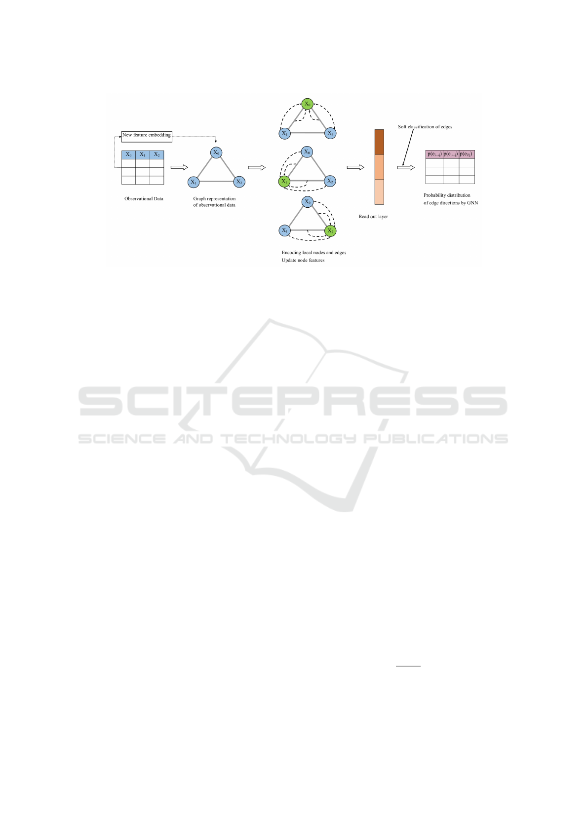
Figure 1: Schematic of the proposed framework. Each node is initialized with statistical features, and each edge with ag-
gregated information-theoretic, statistical, and causal-pairs features (Rashid et al., 2022). The GNN predicts edge directions,
capturing both local and global dependencies to infer the underlying causal graph.
comprehensive feature set that includes both node and
edge features, we can capture a rich representation
of the underlying dependencies and interactions be-
tween variables. The fully connected graph ensures
that all possible relationships are considered, allow-
ing the model to learn from a wide range of potential
causal connections. Furthermore, incorporating the
probability distribution from the causal-pairs model
adds another layer of probabilistic reasoning, enhanc-
ing the model’s ability to infer causal directions accu-
rately. This multi-faceted feature representation en-
ables the GNN to leverage both local and global infor-
mation, leading to more accurate and reliable causal
predictions.
3.2 Developing the Graph Neural
Network (GNN) Model
Graph neural networks (GNNs) are a family of ar-
chitectures that leverage graph structure, node fea-
tures, and edge features to learn dense graph represen-
tations. GNNs employ a neighborhood aggregation
strategy, iteratively updating node representations by
aggregating information from neighboring nodes. For
example, a basic operator for neighborhood informa-
tion aggregation is the element-wise mean.
In our study, we utilize a GNN model as an edge
classifier by training it on synthetic datasets with un-
derlying causal graphs to infer the probability distri-
bution over edge directions through supervised learn-
ing. Although recent works propose more sophis-
ticated GNN variants, we specifically adopt Graph-
SAGE as our backbone due to its scalability and effi-
cient sampling-based message passing, which is par-
ticularly well-suited for large, fully connected graphs.
This choice strikes a balance between computational
efficiency, ease of implementation, and empirical ro-
bustness, rather than architectural novelty.
Starting with a fully connected complete graph,
GraphSAGE enables efficient learning by sampling
and aggregating messages from a subset of neighbors,
improving scalability in message-passing iterations
without compromising model accuracy. This aligns
with our intuition regarding the importance of local
neighborhoods in characterizing conditional indepen-
dences - a key aspect of causal discovery. Although
GraphSAGE is primarily designed to update node fea-
tures based on neighboring node features, we extend it
to incorporate edge features into the message-passing
process, allowing the model to better capture pairwise
dependencies relevant to causal inference. The model
learns a mapping from the edge features (e.g., mu-
tual information, conditional entropy) to edge direc-
tion probabilities, using training graphs with known
causal structure. This replaces the need for dataset-
specific search or constraint satisfaction.
To integrate both node and edge features, we de-
fine the message m
(k)
uv
as a combination of the feature
vectors of nodes u and v at layer (k-1), along with
the edge feature vector e
uv
. The updated equations
for message passing and node feature updates are as
follows:
m
(k)
uv
= CONCAT(h
(k−1)
u
,h
(k−1)
v
,e
uv
) (2)
m
(k+1)
v
=
1
|N(v)|
∑
u∈N(v)
m
(k)
uv
(3)
h
(k+1)
v
= σ
W · CONCAT(h
(k)
v
,m
(k+1)
v
)
(4)
KDIR 2025 - 17th International Conference on Knowledge Discovery and Information Retrieval
340

Here,
• For each neighboring node u of node v, we calcu-
late a message m
(k)
uv
by concatenating the feature
vectors of node u and node v at layer k − 1 along
with the edge feature vector e
uv
.
• The messages m
(k)
uv
from all neighbors u ∈ N(v)
are aggregated by summing them and normalizing
by the number of neighbors |N(v)|. This normal-
ization ensures that contributions from all neigh-
bors are equally weighted.
• The aggregated message m
(k+1)
v
is concatenated
with the current feature vector of node v (h
(k)
v
).
• The concatenated vector is then passed through
a linear transformation defined by the learnable
weight matrix W , followed by a non-linear acti-
vation function σ (e.g., ReLU).
This model captures both local and global depen-
dencies in the graph structure, enhancing the accuracy
of inferred causal relations between nodes consider-
ing their relationships with neighbors. After multiple
rounds of message passing, the final node embeddings
represent each node and edge in the graph, allowing
for the prediction of edge direction probabilities (for-
ward, reverse, or no edge) between any pair of nodes.
3.3 Probabilistic Inference
The edge probabilities predicted by the GNN model
define a distribution over all possible graphs, rather
than directly yielding a single acyclic structure
p(G
DAG
). This probabilistic formulation captures the
inherent uncertainty in causal relationships, allowing
for a more comprehensive representation of potential
causal structures instead of committing to a single de-
terministic graph.
To extract meaningful graph representations from
this probabilistic space, we consider four approaches
as presented in Rashid et al. (2022): (1) Probability
of Graph (PG), which represents the full probability
distribution over directed graphs and can be used to
sample a digraph; (2) Maximum Likelihood Digraph
(MLG), which selects the most probable edge direc-
tions to form a representative structure; (3) Probabil-
ity of DAG (PDAG), which refines the probability dis-
tribution by incorporating acyclicity constraints and
enables sampling of DAGs; and (4) Maximum Like-
lihood DAG (MLDAG), which provides a determin-
istic estimate of the most probable acyclic structure.
The transition from PG/MLG to PDAG/MLDAG is
crucial: while the first two approaches allow cycles,
the latter two explicitly enforce the acyclicity assump-
tion required for valid causal graphs. These meth-
ods progressively refine the estimated causal graph,
ensuring structural validity while balancing proba-
bilistic inference with computational efficiency. This
probabilistic formulation supports multiple inference
strategies, enabling both flexible sampling and strict
acyclicity enforcement. It contrasts with determin-
istic methods like PC or GES, which return only
a single output graph without uncertainty estimates
and require full recomputation per dataset. For clar-
ity, we briefly outline each approach below and refer
to Rashid et al. (2022) for detailed algorithmic deriva-
tions and proofs.
Sample Digraph (PG). The first and most intuitive
approach is to construct the probability distribution
of a digraph G using the maximum entropy princi-
ple. After computing the probability distributions of
causal relationships between node pairs or edge direc-
tions, this method assumes that edge directions are in-
dependent, resulting in a straightforward formulation
(Eq. 5).
p(G| f ) =
∏
i< j
p(e
i j
| f ) (5)
Maximum Likelihood Digraph (MLG). Given the
above naive distribution over digraphs, one can ex-
tract a single representative structure by selecting the
edge directions with the highest probabilities. This
leads to the maximum likelihood digraph, which rep-
resents the most likely structure according to Eq. 6.
G
ML
= argmax
G
p(G| f ) (6)
Note that the samples from the probability distri-
bution, Eq. 5, and the maximum likelihood digraph in
Eq. 6, are digraphs with no guarantees of acyclicity.
Sample DAG (PDAG). A more principled ap-
proach refines the naive distribution by explicitly en-
suring acyclicity of the generated graphs. Rather than
independently sampling edge directions, this method
incorporates DAG constraints by marginalizing over
the topological ordering π of vertices, as shown in
Eq. 7:
p(G| f ,DAG) =
∑
π
p(G| f ,DAG,π)p(π| f ) (7)
Due to the computational intractability of
marginalizing over π, we approximate the probability
of DAGs by conditioning on the maximum likelihood
topological ordering, π
ML
. This leads to the following
approximation:
p(G| f ,DAG,π
ML
) =
∏
π
−1
ML
[i]<π
−1
ML
[ j]
p(e
i→ j
| f ) (8)
From Observations to Causations: A GNN-Based Probabilistic Prediction Framework for Causal Discovery
341

Furthermore, we approximate the maximum like-
lihood topological ordering, π
ML
, by performing a
topological sort on the Maximum Spanning DAG
(MSDAG) (Schluter, 2014), which is computed from
the induced weighted graph G
A
, defined by the prob-
abilities of causal relations:
π
ML
= argmax
π
p(π| f ) ≈ toposort(MSDAG(G
A
)) (9)
In practice, to compute the topological ordering
from the MSDAG of G
A
, we follow the procedure in-
troduced by McDonald and Pereira (2006): first con-
structing a maximum spanning tree, then incremen-
tally adding edges in descending order of weights
while ensuring acyclicity at each step.
Maximum Likelihood DAG (MLDAG). Extend-
ing the MLG approach to enforce acyclicity, the max-
imum likelihood DAG provides a deterministic rep-
resentation of the most probable causal structure. In-
stead of selecting the highest-probability edges inde-
pendently, this method ensures acyclicity by incorpo-
rating the DAG constraints introduced in the previous
approach. In other words, edges are selected in order
of probability, but only if they do not introduce a cycle
with respect to the current partial ordering. Thus the
resulting graph is constructed by selecting the most
probable edges while maintaining a valid topological
ordering, as formulated in Eq. 10.
G
DAG
≈ argmax
G
p(G| f ,DAG,π
ML
) (10)
4 EXPERIMENTS
To evaluate the effectiveness of our proposed prob-
abilistic inference methods, we conduct experiments
on synthetic, benchmark, and real-world datasets.
We compare our approaches, GNN-PG (sample di-
graph from the probability distribution), GNN-MLG
(maximum likelihood estimate digraph), GNN-PDAG
(sample DAG from the probability distribution), and
GNN-MLDAG (DAG using the maximum likelihood
estimate), against both traditional and recent causal
discovery methods.
Specifically, we benchmark our methods against
classical algorithms such as PC (Spirtes et al.,
2001) and GES (Chickering, 2002), as well as re-
cent approaches including LiNGAM (Shimizu et al.,
2006), DAG-GNN (Yu et al., 2019), NOTEARS-
MLP (Zheng et al., 2020), DiBS (Lorch et al., 2021),
and DAGMA (Bello et al., 2022). For PC, GES,
and LiNGAM, we use publicly available implemen-
tations
1,2,3
, while for DAG-GNN, NOTEARS-MLP,
DiBS, and DAGMA, we follow the implementations
provided by the respective authors
4,5,6,7
. We use de-
fault hyperparameter settings for all methods to en-
sure a fair comparison.
4.1 Datasets
Synthetic Data. We generated synthetic data to
train our GNN model on causal graph estimation, pro-
ducing 200 graphs with 72 different combinations of
nodes (d = [10,20,50,100]), edges (e = [1d, 2d,4d]),
data samples per node (n = [500,1000,2000]), and
graph models (Erdos-Renyi and Scale-Free). Non-
linear data samples were generated similarly to
the NOTEARS-MLP implementation, with random
graph structures and ground truth for training. The
process for generating synthetic test data follows the
methodology outlined in Rashid et al. (2022), where
160 types of graph combinations were considered,
each with varying numbers of nodes, edges, graph
types, and data samples per node.
CSuite Data. In addition to our synthetic test
datasets, we employed five benchmark datasets from
Microsoft CSuite, a collection designed for evaluating
causal discovery and inference algorithms (Geffner
et al., 2022). The CSuite data is generated from
well-defined hand-crafted structural equation models
(SEMs), which serve to test various aspects of causal
inference methodologies. The five datasets utilized in
our study are: large backdoor (9 nodes, 10 edges);
weak arrows (9 nodes, 15 edges); mixed simpson (4
nodes, 4 edges); nonlin simpson (4 nodes, 4 edges);
symprod simpson (4 nodes, 4 edges);. Each dataset
includes 6000 data samples, and a corresponding
ground truth graph, providing a basis for performance
evaluation.
Real-World Data. We used the dataset from Sachs
et al. (2005), based on protein expression levels. This
dataset is widely used due to its consensus ground
truth of the graph structure, consisting of 11 protein
nodes and 17 edges representing the protein signaling
network. We aggregated 9 data files, resulting in a
sample size of 7466 for our experiments.
1
PC: https://github.com/keiichishima/pcalg
2
GES: https://github.com/juangamella/ges
3
LiNGAM: https://lingam.readthedocs.io/en/latest
4
DAG-GNN: https://github.com/fishmoon1234/DAG-
GNN
5
NOTEARS-MLP: https://github.com/xunzheng/notears
6
DiBS: https://github.com/larslorch/dibs
7
DAGMA: https://github.com/kevinsbello/dagma
KDIR 2025 - 17th International Conference on Knowledge Discovery and Information Retrieval
342

4.2 Metrics
We evaluate the quality of the inferred causal graphs
using True Positive Rate (TPR), False Positive Rate
(FPR), and Structural Hamming Distance (SHD). A
lower SHD and FPR indicate better performance,
while a higher TPR is preferable. To ensure a fair
comparison, these metrics are computed consistently
across all methods, following the procedures used in
prior evaluations of PC, GES, and NOTEARS-MLP.
GNN-based and CausalPairs-based methods adhere to
the implementation framework described in Rashid
et al. (2022).
4.3 Results
Table 1 showcases the performance of our GNN-
based methods on 80 Scale-Free (SF) and 80 Erdos-
Renyi (ER) graph structures. Our methods consis-
tently outperform traditional and recent approaches,
demonstrating improved recovery of causal structures
through reduced Structural Hamming Distance (SHD)
and increased True Positive Rate (TPR). Key observa-
tions across both graph structures include:
1. Our GNN-based methods, especially GNN-
PDAG and GNN-MLDAG, consistently achieve
lower SHD and higher TPR values compared to
CausalPairs methods; traditional methods such as
PC and GES; and DiBS. They also perform fa-
vorably or better than advanced methods such
as LiNGAM, DAG-GNN, NOTEARS-MLP, and
DAGMA. Notably, they significantly improve
TPR while maintaining low SHD.
2. The GNN-MLG method significantly minimizes
false positive causal relationships, but at the cost
of a lower TPR. Other GNN-based methods bal-
ance TPR and FPR.
3. Enforcing DAG constraints in GNN-PDAG and
GNN-MLDAG improves performance metrics
relative to GNN-PG and GNN-MLG, highlight-
ing the benefit of integrating global structural in-
formation to enhance accuracy.
Figure 2 presents a comprehensive comparison of
the Structural Hamming Distance (SHD), True Pos-
itive Rate (TPR), and False Positive Rate (FPR) per-
formance metrics for different methods on 160 SF and
ER graphs with node-to-edge ratios of 1:1 and 1:4.
Our GNN-based methods, specifically GNN-
PDAG and GNN-MLDAG, consistently achieve
lower SHD values than traditional methods (PC and
GES), CausalPairs methods, and advanced methods
(NOTEARS-MLP, DAG-GNN, and DAGMA). No-
tably, our proposed methods (GNN-PG, GNN-PDAG,
and GNN-MLDAG) demonstrate significantly higher
TPRs than all other methods, indicating improved
accuracy in identifying true causal relationships.
GNN-PDAG and GNN-MLDAG exhibit robust per-
formance across both sparse (1:1) and dense (1:4)
graphs, showcasing their ability to accurately recover
causal structures with fewer errors. The improvement
is more pronounced in denser graphs (1:4 node-to-
edge ratio), showing promise in handling complex,
highly connected networks.
Tables 2 present the results of applying our meth-
ods to five datasets from the Microsoft CSuite. Our
methods achieve significantly lower SHD, higher
TPR, and lower FPR compared to all other methods,
demonstrating the robustness and generalizability of
our GNN-based framework across diverse datasets.
Compared to the synthetic datasets presented in Ta-
ble 1, the Microsoft CSuite datasets have fewer nodes
and edges. Additionally, the three smaller datasets
from Microsoft CSuite allow us to demonstrate the
method’s capability to recover various graph struc-
tures learned directly from data.
In these datasets, which include graphs with four
nodes and four edges, our methods accurately iden-
tified V structures such as A → B ← C. This abil-
ity to capture fork or collider structures highlights the
method’s precision in determining causal directions
and understanding interactions between variables. We
also observed that in datasets like mixed simpson and
nonlin simpson, with confounder structures such as
B ← A → C, our methods demonstrated the ability
to recognize common causes affecting multiple out-
comes. Chain structures like A → B → C were also
accurately recovered, showcasing the capability to
model sequential causal relationships. For instance,
among two of these datasets, our GNN-based meth-
ods achieved a SHD score of 0 and a TPR score of
1, perfectly identifying the true graph, and validating
our methods’ effectiveness in learning complex causal
structures.
Notably, as shown in Figure 3, our GNN-based
methods not only identified the true graph structure
but also avoided predicting extraneous edges. In con-
trast, while CausalPairs methods were able to identify
the true edges, they also predicted all possible edges,
leading to higher false positives. This underscores the
precision of our GNN-based approach in distinguish-
ing true causal relationships from spurious ones.
In Table 3, our methods, particularly GNN-PG
and GNN-MLDAG, demonstrate strong performance
on the real-world protein network dataset, accu-
rately predicting edge counts. Notably, they out-
perform LiNGAM, DiBS and GES in terms of cor-
rect edge predictions, and even match or surpass
From Observations to Causations: A GNN-Based Probabilistic Prediction Framework for Causal Discovery
343
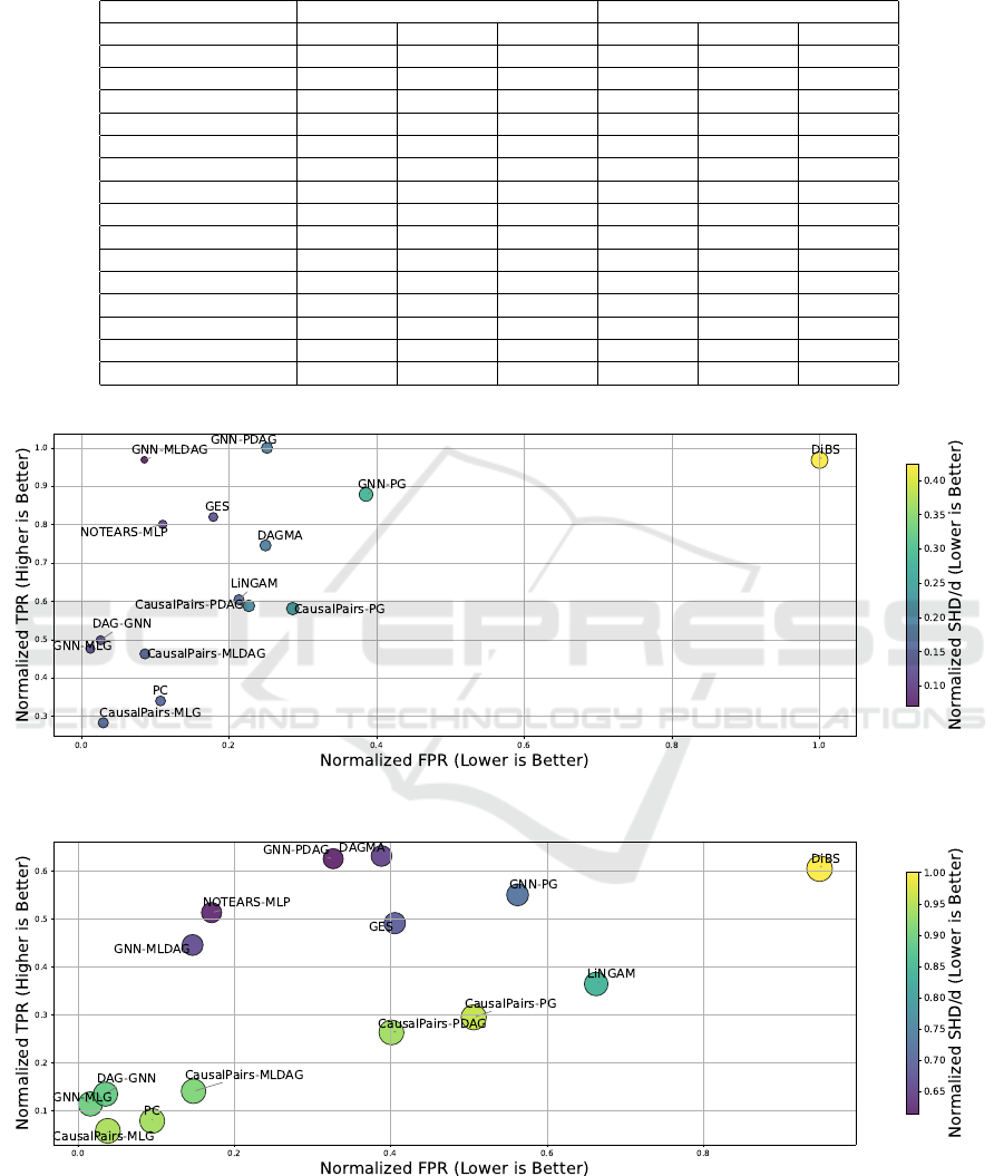
Table 1: Comparison of edge probability model trained on GNN framework. The means and standard errors of the perfor-
mance metrics are based on the 80 Scale-Free (SF) and 80 Erdos-Renyi (ER) graph structures in the test data.
Dataset Name → Scale-Free (SF) Erdos-Renyi (ER)
Method ↓ — Metrics → SHD/d TPR FPR SHD/d TPR FPR
GNN PG 1.88±0.08 0.51±0.02 0.30±0.01 2.08±0.11 0.52±0.02 0.52±0.06
GNN MLG 1.85±0.13 0.20±0.02 0.01±0.00 2.17±0.17 0.25±0.02 0.01±0.00
GNN PDAG 1.55±0.07 0.56±0.02 0.19±0.01 1.75±0.11 0.61±0.03 0.28±0.03
GNN MLDAG 1.40±0.11 0.48±0.03 0.08±0.01 1.66±0.15 0.54±0.03 0.13±0.02
CausalPairs PG 2.02±0.12 0.31±0.01 0.26±0.02 2.38±0.14 0.39±0.02 0.72±0.10
CausalPairs MLG 1.97±0.13 0.12±0.01 0.03±0.01 2.32±0.17 0.15±0.02 0.07±0.01
CausalPairs PDAG 1.96±0.12 0.30±0.01 0.21±0.02 2.30±0.15 0.38±0.02 0.61±0.09
CausalPairs MLDAG 1.88±0.13 0.20±0.01 0.09±0.01 2.18±0.16 0.28±0.02 0.29±0.05
PC 1.93±0.15 0.17±0.02 0.08±0.01 2.40±0.21 0.17±0.02 0.22±0.04
GES 1.43±0.11 0.51±0.03 0.26±0.04 1.78±0.13 0.48±0.02 0.87±0.15
LiNGAM 1.68±0.11 0.35±0.02 0.34±0.04 1.97±0.13 0.43±0.02 1.04±0.17
DAG-GNN 1.75±0.12 0.24±0.02 0.02±0.00 2.10±0.17 0.27±0.02 0.06±0.00
NOTEARS 1.36±0.11 0.47±0.02 0.12±0.02 1.33±0.10 0.58±0.02 0.32±0.06
DiBS 2.51±0.08 0.32±0.02 0.91±0.25 2.78±0.10 0.34±0.02 0.38±0.06
DAGMA 1.39±0.09 0.54±0.02 0.21±0.02 1.80±0.11 0.51±0.02 0.65±0.10
(a) Node : Edge (1:1)
(b) Node : Edge (1:4)
Figure 2: Comparison of normalized Structural Hamming Distance (SHD/d), True Positive Rate (TPR), and False Positive
Rate (FPR) across methods on Erdos-Renyi (ER) and Scale-Free (SF) graphs, evaluated for both sparse (1:1) and dense
(1:4) node-to-edge ratios. Metrics are computed as the mean and standard error over 80 randomly generated graphs for each
condition.
KDIR 2025 - 17th International Conference on Knowledge Discovery and Information Retrieval
344
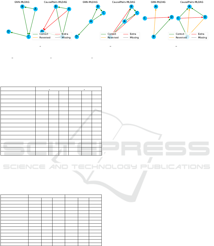
(a) nonlin simpson (b) symprod simpson (c) mixed simpson
Figure 3: Performance comparison between GNN-based methods and CausalPairs methods on smaller CSuite datasets: (a)
nonlin simpson, (b) symprod simpson, and (c) mixed simpson. The plots illustrate the number of correct, reversed, extra, and
missing edges for each method with respect to the ground truth graphs.
Table 2: Comparison of GNN-based edge probability model
(trained on synthetic train data) on the Microsoft CSuite
datasets.
Dataset Name → large backdoor weak arrows
Method ↓ — Metrics → SHD/d TPR FPR SHD/d TPR FPR
GNN PG 0.59 0.42 0.20 0.56 0.66 0.24
GNN MLG 0.68 0.32 0.17 0.82 0.51 0.09
GNN PDAG 0.56 0.44 0.19 0.67 0.60 0.29
GNN MLDAG 0.55 0.44 0.18 0.66 0.60 0.28
CausalPairs PG 2.42 0.88 0.80 2.24 0.85 0.93
CausalPairs MLG 1.77 0.88 0.55 1.89 0.82 0.68
CausalPairs PDAG 2.28 0.97 0.75 2.06 0.95 0.85
CausalPairs MLDAG 2.14 0.96 0.70 1.97 0.94 0.81
PC 1.00 0.53 0.29 0.89 0.44 0.22
GES 1.33 0.67 0.67 0.88 0.88 0.37
LiNGAM 2.22 0.20 0.91 1.67 0.22 0.56
DAG-GNN 0.89 0.53 0.05 0.67 0.44 0.04
NOTEARS 1.00 0.47 0.19 0.89 0.44 0.19
DiBS 3.33 0.50 0.94 3.11 0.43 0.97
DAGMA 1.22 0.33 0.37 1.78 0.20 0.52
Table 3: Comparison of GNN-based edge probability model
(trained on synthetic train data) on the protein network
datasets (Sachs et al., 2005). DAG-GNN (Yu et al.,
2019) and NOTEARS-MLP (Zheng et al., 2020) results
for non-standardized data are reported from the original
manuscripts.
Dataset Type → Standardized Non-standardized
Method ↓ — Metrics → Predicted Correct Reversed Predicted Correct Reversed
GNN PG 19.68 6.60 6.98 19.40 5.86 7.79
GNN MLG 12.07 5.13 5.64 13.81 5.48 6.86
GNN PDAG 17.09 6.96 5.81 16.74 4.14 8.62
GNN MLDAG 14.12 6.96 5.81 12.54 4.71 7.77
CausalPairs PG 36.14 6.70 7.77 38.01 6.21 8.26
CausalPairs MLG 9.82 3.04 4.26 10.41 1.52 4.04
CausalPairs PDAG 33.16 7.42 6.62 34.81 6.47 7.49
CausalPairs MLDAG 18.48 4.91 5.41 20.60 4.71 6.32
GES 34.00 5.50 9.50 34.00 5.50 9.50
LiNGAM 36.00 4.00 11.00 36.00 4.00 11.00
DAG-GNN 6.00 1.00 5.00 18.00 8.00 3.00
NOTEARS 42.33 5.83 7.18 13.00 7.00 3.00
DiBS 46.00 7.00 7.00 50.00 8.00 9.00
DAGMA 11.00 3.00 5.00 7.00 5.50 1.50
the performance of recent methods like NOTEARS-
MLP, DAG-GNN, and DAGMA. The incorporation
of global structural information through GNNs en-
ables accurate edge prediction, while our approach
also shows improved directional accuracy, as evident
from the lower number of reversed edges achieved by
GNN-MLDAG and GNN-PG.
A notable aspect is that DAG-GNN and
NOTEARS-MLP exhibit sensitivity to data scaling,
with performance variations between standardized
and non-standardized data. This sensitivity arises
because their continuous optimization processes
can be disrupted by changes in data magnitude
and distribution. Additionally, LiNGAM, which
is designed for non-Gaussian linear models, may
struggle with the non-linear relationships present
in the protein network dataset. In contrast, our
GNN-based methods show consistent performance
across both standardized and non-standardized
datasets, demonstrating robustness to data scaling.
This robustness is attributed to the effective capture
and utilization of both local and global structural
information by GNNs.
5 CONCLUSIONS
In this work, we introduce a probabilistic causal
discovery framework that leverages Graph Neu-
ral Networks (GNNs) within a supervised learning
paradigm. Our approach, trained exclusively on syn-
thetic datasets, effectively generalizes to real-world
datasets without requiring additional training.
By exploiting global structural information, our
method addresses key limitations of traditional causal
discovery techniques, significantly enhancing pre-
cision in learning causal graphs. Through inte-
grated node and edge features, our GNN-based model
captures complex dependency structures, facilitating
more accurate and reliable causal inference.
Future research directions will include explic-
itly incorporating acyclicity constraints into the GNN
framework to potentially enhance the robustness and
accuracy of inferred causal structures. Additionally,
investigating advanced GNN architectures may fur-
ther optimize our method’s performance.
From Observations to Causations: A GNN-Based Probabilistic Prediction Framework for Causal Discovery
345

ACKNOWLEDGEMENTS
The research was sponsored by the Army Research
Office and was accomplished under Grant Number
W911NF-22-1-0035. The views and conclusions con-
tained in this document are those of the authors and
should not be interpreted as representing the official
policies, either expressed or implied, of the Army
Research Office or the U.S. Government. The U.S.
Government is authorized to reproduce and distribute
reprints for Government purposes notwithstanding
any copyright notation herein.
REFERENCES
Behnam, A. and Wang, B. (2024). Graph neural network
causal explanation via neural causal models. In Euro-
pean Conference on Computer Vision, pages 410–427.
Springer.
Bello, K., Aragam, B., and Ravikumar, P. (2022).
DAGMA: Learning DAGs via M-matrices and a Log-
Determinant Acyclicity Characterization. In Advances
in Neural Information Processing Systems.
Bouckaert, R. R. (1993). Probabilistic network construc-
tion using the minimum description length principle.
In European conference on symbolic and quantitative
approaches to reasoning and uncertainty, pages 41–
48. Springer.
Brouillard, P., Lachapelle, S., Lacoste, A., Lacoste-Julien,
S., and Drouin, A. (2020). Differentiable causal dis-
covery from interventional data. Advances in Neural
Information Processing Systems, 33:21865–21877.
Chickering, D. M. (2002). Optimal structure identification
with greedy search. Journal of machine learning re-
search, 3(Nov):507–554.
Fonollosa, J. A. (2019). Conditional distribution variability
measures for causality detection. Cause Effect Pairs
in Machine Learning, pages 339–347.
G
´
amez, J. A., Mateo, J. L., and Puerta, J. M. (2011).
Learning bayesian networks by hill climbing: effi-
cient methods based on progressive restriction of the
neighborhood. Data Mining and Knowledge Discov-
ery, 22:106–148.
Gao, H., Yao, C., Li, J., Si, L., Jin, Y., Wu, F., Zheng, C.,
and Liu, H. (2024). Rethinking causal relationships
learning in graph neural networks. In Proceedings of
the AAAI Conference on Artificial Intelligence, vol-
ume 38, pages 12145–12154.
Geffner, T., Antoran, J., Foster, A., Gong, W., Ma, C.,
Kiciman, E., Sharma, A., Lamb, A., Kukla, M.,
Pawlowski, N., Allamanis, M., and Zhang, C. (2022).
Deep end-to-end causal inference. arXiv preprint
arXiv:2202.02195.
Hamilton, W., Ying, Z., and Leskovec, J. (2017). Inductive
representation learning on large graphs. Advances in
neural information processing systems, 30.
Heckerman, D., Geiger, D., and Chickering, D. M. (1995).
Learning bayesian networks: The combination of
knowledge and statistical data. Machine learning,
20:197–243.
Jiang, W., Liu, H., and Xiong, H. (2023). When
graph neural network meets causality: Opportuni-
ties, methodologies and an outlook. arXiv preprint
arXiv:2312.12477.
Job, S., Tao, X., Cai, T., Xie, H., Li, L., Li, Q., and Yong,
J. (2025). Exploring causal learning through graph
neural networks: An in-depth review. Wiley Interdis-
ciplinary Reviews: Data Mining and Knowledge Dis-
covery, 15(2):e70024.
Kipf, T. N. and Welling, M. (2016). Semi-supervised clas-
sification with graph convolutional networks. arXiv
preprint arXiv:1609.02907.
Koller, D. and Friedman, N. (2009). Probabilistic graphical
models: principles and techniques. MIT press.
Lacerda, G., Spirtes, P. L., Ramsey, J., and Hoyer,
P. O. (2012). Discovering cyclic causal models by
independent components analysis. arXiv preprint
arXiv:1206.3273.
Li, H., Xiao, Q., and Tian, J. (2020). Supervised whole dag
causal discovery. arXiv preprint arXiv:2006.04697.
Lin, W., Lan, H., and Li, B. (2021). Generative causal ex-
planations for graph neural networks. In International
Conference on Machine Learning, pages 6666–6679.
PMLR.
Lorch, L., Rothfuss, J., Sch
¨
olkopf, B., and Krause, A.
(2021). Dibs: Differentiable bayesian structure learn-
ing. Advances in Neural Information Processing Sys-
tems, 34.
Lorch, L., Sussex, S., Rothfuss, J., Krause, A., and
Sch
¨
olkopf, B. (2022). Amortized inference for causal
structure learning. Advances in Neural Information
Processing Systems, 35:13104–13118.
McDonald, R. and Pereira, F. (2006). Online learning of
approximate dependency parsing algorithms. In 11th
Conference of the European Chapter of the Associa-
tion for Computational Linguistics, pages 81–88.
Mohammadi, A. and Wit, E. C. (2015). Bayesian structure
learning in sparse gaussian graphical models.
Mohan, K., Chung, M., Han, S., Witten, D., Lee, S.-I.,
and Fazel, M. (2012). Structured learning of gaus-
sian graphical models. Advances in neural informa-
tion processing systems, 25.
Ng, I., Zhu, S., Chen, Z., and Fang, Z. (2019). A graph au-
toencoder approach to causal structure learning. arXiv
preprint arXiv:1911.07420.
Ott, S., Imoto, S., and Miyano, S. (2003). Finding opti-
mal models for small gene networks. In Biocomputing
2004, pages 557–567. World Scientific.
Pearl, J. (2019). The seven tools of causal inference, with
reflections on machine learning. Communications of
the ACM, 62(3):54–60.
Peters, J., Janzing, D., and Sch
¨
olkopf, B. (2017). Elements
of causal inference: foundations and learning algo-
rithms. The MIT Press.
KDIR 2025 - 17th International Conference on Knowledge Discovery and Information Retrieval
346

Rashid, R., Chowdhury, J., and Terejanu, G. (2022). From
causal pairs to causal graphs. In 2022 21st IEEE In-
ternational Conference on Machine Learning and Ap-
plications (ICMLA), pages 802–807. IEEE.
Reisach, A., Seiler, C., and Weichwald, S. (2021). Beware
of the simulated dag! causal discovery benchmarks
may be easy to game. Advances in Neural Information
Processing Systems, 34:27772–27784.
Sachs, K., Perez, O., Pe’er, D., Lauffenburger, D. A., and
Nolan, G. P. (2005). Causal protein-signaling net-
works derived from multiparameter single-cell data.
Science, 308(5721):523–529.
Schluter, N. (2014). On maximum spanning dag algorithms
for semantic dag parsing. In Proceedings of the ACL
2014 Workshop on Semantic Parsing, pages 61–65.
Shimizu, S., Hoyer, P. O., Hyv
¨
arinen, A., Kerminen, A.,
and Jordan, M. (2006). A linear non-gaussian acyclic
model for causal discovery. Journal of Machine
Learning Research, 7(10).
Singh, K., Gupta, G., Vig, L., Shroff, G., and Agarwal, P.
(2017). Deep convolutional neural networks for pair-
wise causality. arXiv preprint arXiv:1701.00597.
Spirtes, P., Glymour, C., and Scheines, R. (2001). Causa-
tion, prediction, and search. MIT press.
Tsamardinos, I., Brown, L. E., and Aliferis, C. F. (2006).
The max-min hill-climbing bayesian network struc-
ture learning algorithm. Machine learning, 65:31–78.
Velickovic, P., Cucurull, G., Casanova, A., Romero, A., Lio,
P., Bengio, Y., et al. (2017). Graph attention networks.
stat, 1050(20):10–48550.
Waikhom, L. and Patgiri, R. (2023). A survey of graph neu-
ral networks in various learning paradigms: methods,
applications, and challenges. Artificial Intelligence
Review, 56(7):6295–6364.
Yu, Y., Chen, J., Gao, T., and Yu, M. (2019). Dag-gnn: Dag
structure learning with graph neural networks. In In-
ternational Conference on Machine Learning, pages
7154–7163. PMLR.
Ze
ˇ
cevi
´
c, M., Dhami, D. S., Veli
ˇ
ckovi
´
c, P., and Kersting, K.
(2021). Relating graph neural networks to structural
causal models. arXiv preprint arXiv:2109.04173.
Zhao, S., Prapas, I., Karasante, I., Xiong, Z., Papoutsis, I.,
Camps-Valls, G., and Zhu, X. X. (2024). Causal graph
neural networks for wildfire danger prediction. arXiv
preprint arXiv:2403.08414.
Zheng, X., Aragam, B., Ravikumar, P. K., and Xing, E. P.
(2018). Dags with no tears: Continuous optimization
for structure learning. Advances in neural information
processing systems, 31.
Zheng, X., Dan, C., Aragam, B., Ravikumar, P., and Xing,
E. (2020). Learning sparse nonparametric dags. In In-
ternational Conference on Artificial Intelligence and
Statistics, pages 3414–3425. Pmlr.
Zhou, J., Cui, G., Hu, S., Zhang, Z., Yang, C., Liu, Z.,
Wang, L., Li, C., and Sun, M. (2020). Graph neu-
ral networks: A review of methods and applications.
AI open, 1:57–81.
APPENDIX
List of Node and Edge Features
Node Features
The following features are extracted for each node in
the graph, capturing individual statistical properties
that are independent of relationships with other nodes.
• Min, Max
• Numerical Type
• Number of Unique Samples
• Ratio of Unique Samples
• Log of Number of Samples
• Normalized Entropy
• Normalized Entropy Baseline
• Uniform Divergence
• Discrete Entropy
• Normalized Discrete Entropy
• Skewness, Kurtosis
Edge Features
This section provides a comprehensive list of edge
features used in our framework, grouped by type,
which capture statistical and information-theoretic
relationships between pairs of nodes, emphasizing
causal relationships or dependencies.
Information-Theoretic Features
• Mutual Information and Related Measures:
– Discrete Joint Entropy between nodes
– Normalized Discrete Joint Entropy between
nodes
– Discrete Mutual Information between nodes
– Adjusted Mutual Information between nodes
– Normalized Discrete Mutual Information
• Conditional Entropy:
– Discrete Conditional Entropy for each node
pair
• Divergence Measures:
– Uniform Divergence for individual nodes
– Subtracted Divergence between nodes
From Observations to Causations: A GNN-Based Probabilistic Prediction Framework for Causal Discovery
347

Regression-Based Features
• Polynomial Fitting:
– Polynomial Fit between nodes
– Polynomial Fit Error between nodes
– Subtracted Polynomial Fit between nodes
• Error Metrics:
– Normalized Error Probability for each node
pair
– Subtracted Normalized Error Probability be-
tween nodes
Statistical Distribution Metrics
• Moment-Based Metrics:
– Second-order moments (Moment21) between
nodes
– Third-order moments (Moment31) between
nodes
– Subtracted moments and their absolute values
• Conditional Distribution Metrics:
– Entropy variance across node pairs
– Skewness variance across node pairs
– Kurtosis variance across node pairs
Correlation Measures
• Pearson Correlation:
– Pearson Correlation Coefficient between nodes
– Absolute Pearson Correlation
Node Pair Comparisons
• Sample-Based Comparisons:
– Maximum, minimum, and difference in the
number of unique samples between nodes
• Entropy Comparisons:
– Maximum, minimum, and difference in nor-
malized entropy between nodes
Other Features
• Hilbert-Schmidt Independence Criterion (HSIC)
between nodes
• Subtracted Information-Geometric Causal Infer-
ence (IGCI) values
• Absolute differences in kurtosis between nodes
• Other advanced metrics derived from normalized
probabilities and variance measures
KDIR 2025 - 17th International Conference on Knowledge Discovery and Information Retrieval
348
