Optimal Camera Placement for 6D Head Pose Estimation
Harshita Soni, Nikhil Tirumala and Aratrik Chattopadhyay
Mercedes Benz R&D India, Bengaluru, India
Keywords:
Optimal Camera Placement, Visibility, Binary Integer Programming.
Abstract:
Multi-view systems for 6D head pose estimation have applications in human-computer interaction (HCI),
virtual reality, 3D reconstruction etc. In a multi-view system, visibility of facial landmarks is essential for ac-
curately regressing 2D landmarks, which are then triangulated to get 3D fiducials. From these 3D fiducials, the
6D head pose is mathematically derived. Optimal camera placement (OCP) is vital for achieving precise pose
estimation. OCP can be formulated as a constrained optimization problem that can be solved using Binary
Integer Programming. We redefine two key aspects: the visibility criteria and the camera search space. Our
visibility algorithm employs a parametric head model to track fiducials, achieving more precise results than
ground truth of CMU(Carnegie Mellon University) Panoptic dataset. Additionally, we geometrically optimize
the camera search space, deviating from the baseline of uniformly arranged cameras. Through rigorous exper-
imentation, we prove that not only does this refined search space reduce execution time, but also improves the
optimality of the solution, giving 99.9% visibility coverage. We also introduce a heuristic method that reduces
the constraint-building time from 27 seconds to just 0.07 seconds per control point, while maintaining concise
solutions with minimal effects on visibility metrics.
1 INTRODUCTION
6D head pose estimation includes three degrees of
freedom for rotation (yaw, pitch, roll) and three for
translation (X, Y, Z). Multi-view systems for 6D head
pose estimation have various applications across dif-
ferent fields. In AR/VR, head pose estimation en-
hances the immersive experience by ensuring virtual
objects align correctly with the user’s perspective. Se-
curity applications are equipped with multi-camera
surveillance systems where head pose estimation can
be used to analyze the behavior and intentions of in-
dividuals in surveillance footage. Additionally, such
systems can be used for ground truth data collection,
like the public dataset, CMU Panoptic [(Joo et al.,
2016)], using data captured to train deep learning
models.
6D head pose estimation is mathematically de-
rived from 3D landmarks of a set of critical points
in a human face, called fiducials, like eye corners,
mouth corners, nose-tip, etc. Fiducials form the back-
bone of most of the downstream functionalities of
such a multi-view system. Fiducials are triangulated
from their 2D landmarks in multiple camera views.
2D facial landmark regression from an image is a
well-known problem that has been addressed using
both traditional computer vision techniques and deep
learning methods. To summarize, the precision of an
end-to-end multi-view system depends on the avail-
ability of a certain minimum number of clear image
views for the 2D landmark regressor to regress on
confidently. Hence, an optimal placement of cameras
is essential for the seamless functioning of a multi-
view system.
The concept of optimal camera placement (OCP)
was outlined by (Chv
´
atal, 1975) in the art gallery
problem in 1975. It aims to determine the minimum
number of guards (or cameras) needed to cover an en-
tire area.
OCP for surveillance applications does not require
tracking objects in 3D. In the case of OCP for 3D ob-
jects, in most use cases, the object is static and in a
fixed, known position and orientation. In this work,
we solve OCP for an application where the target has
continuous changes in 6D pose. Also, we have a strin-
gent requirement of having the selected fiducials of
the object to be visible in all the 6D poses in at least
two cameras. This makes the OCP for a 3D-object-
in-motion a more challenging task.
Another aspect that complicates the visibility
computation in our case is that the human head is a
complex manifold. The visibility of the fiducials is
82
Soni, H., Tirumala, N. and Chattopadhyay, A.
Optimal Camera Placement for 6D Head Pose Estimation.
DOI: 10.5220/0013715100003982
Paper published under CC license (CC BY-NC-ND 4.0)
In Proceedings of the 22nd International Conference on Informatics in Control, Automation and Robotics (ICINCO 2025) - Volume 1, pages 82-92
ISBN: 978-989-758-770-2; ISSN: 2184-2809
Proceedings Copyright © 2025 by SCITEPRESS – Science and Technology Publications, Lda.

sensitive to small changes in head position and orien-
tation, leading to self-occlusion.
The OCP can be solved using two main ap-
proaches: an iterative method, which is not al-
ways optimal, and binary integer programming (BIP),
which guarantees an optimal solution.
Finding an optimal solution using BIP is an NP-
hard problem. Optimization of any of the inputs to
BIP would reduce computation time and allow for
the quick arrival of a solution. This is overlooked
in most previous works, where they merely discretize
the search space into uniform grids. This work shows
that initializing the search space geometrically leads
to reduced computation time and an optimal solution.
We also show that our geometric approach makes the
solution generic, which can be adapted to any larger
3D environment.
The end-to-end pipeline could be computationally
intensive due to framing and solving the constraints.
In this work, we propose an alternate way to precom-
pute and approximate the visibility to save time dur-
ing execution. To summarize, the contributions of our
paper are:
1. We present an algorithm to check the visibility
of fiducials and model self-occlusion for a human
head.
2. We propose an initialization technique for cam-
era search space that drastically reduces the search
space and execution time and optimizes the solu-
tion.
3. We propose an approach to reduce the execution
time by approximating the visibility.
4. We show that camera solutions obtained from our
method can be flexibly fitted to any larger, arbi-
trarily shaped 3D environment.
5. We show the superiority of our method over the
baseline on multiple test metrics.
The paper reviews related work in section 2. Sec-
tion 3 covers the problem statement, including the vis-
ibility model (3.1), OCP formulation (3.2), and cam-
era search space optimization (3.3). Visibility approx-
imation is discussed in section 3.4. Methodologies
are evaluated in section 4, with experiments detailed
in section 5. The paper concludes with key findings
in section 6.
2 RELATED WORK
There has been a lot of work in the domain of optimal
camera placement (OCP) after its origin from the art
gallery problem [(O’Rourke, 1993)].
(H
¨
orster and Lienhart, 2006) has presented the op-
timal camera configuration as an integer linear pro-
gramming problem, which can incorporate different
constraints and cost functions pertinent to a particular
application. They approximate the continuous camera
space by sampling the positions and poses. The visi-
bility model is an essential part of OCP, the definition
of which changes based on the application. [(H
¨
orster
and Lienhart, 2006), (Bettahar et al., 2014)] defined
visibility as the field of view of a camera which is
taken to be a 2D fixed-size triangle, while the visi-
bility in (Zhao et al., 2008) is based on the projected
length of the tag in the image plane. (Puligandla and
Lon
ˇ
cari
´
c, 2022) figures the visibility of a control point
in a camera by checking its presence in the five planes
of the FoV pyramid of the camera. The visible point
analysis technique of (Zhang et al., 2021) is based on
a Hidden Point Removal (HPR) approach. Most of
these visibility models are applicable for tracking ob-
jects or tags, and some have been simplified to 2D.
Given our use case of 6D head pose estimation, track-
ing of 3D facial landmarks cannot be done by 2D-
based projection methods. In contrast, a 3D-based
method like HPR is applicable but susceptible to mis-
classification errors around regions of high local cur-
vature.
[(Zhao et al., 2008), (Liu et al., 2014), (Betta-
har et al., 2014), (Puligandla and Lon
ˇ
cari
´
c, 2022)]
uniformly divide the camera configuration space into
grids and populate the camera search space by placing
cameras in those grids. (Zhang et al., 2015) adopts
the technique of local optimization of a single cam-
era, followed by iterative addition of cameras to cap-
ture the uncovered surfaces, not ensuring optimality
of the overall solution. (Zhang et al., 2021) employs
a genetic algorithm for global optimization of camera
configurations.
3 OCP FOR MULTI-VIEW
SYSTEM
3.1 Visibility Model
We use an off-the-shelf 3D head parametric model
that defines a human head and neck with N
v
ver-
tices and N
f
faces or triangles. The head model
is used to model visibility of a fiducial in a cam-
era. All the cameras are assumed to be pinhole.
Let P = {P
1
,P
2
,...,P
N
v
} be the set of vertices, and
F = {F
1
,F
2
,...,F
N
f
} be the set of triangles in the
head mesh. Fiducial points (N
K
) are some critical
points subsetted from P. Let K = {k
1
,k
2
,...,k
N
K
}
Optimal Camera Placement for 6D Head Pose Estimation
83

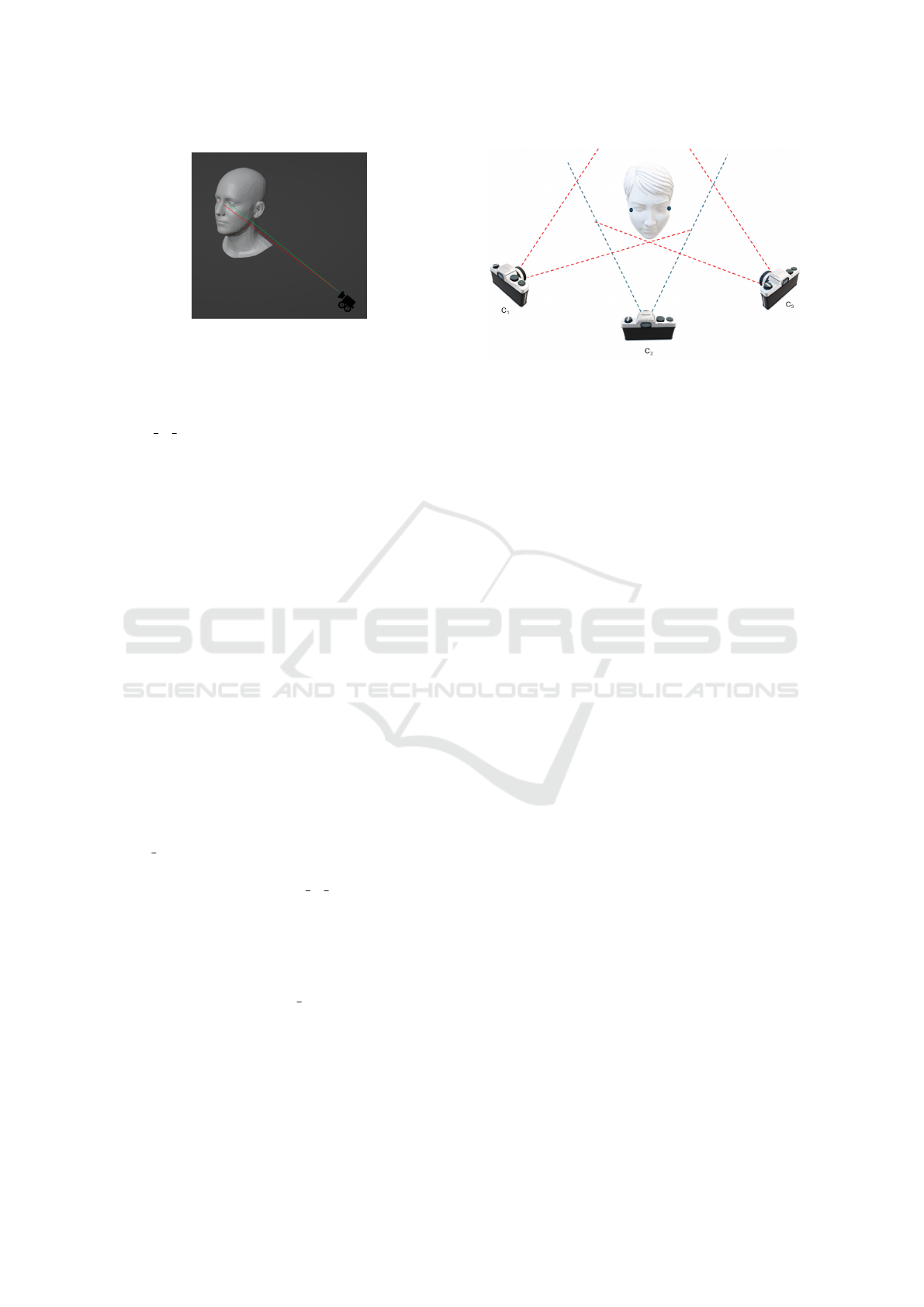
Figure 1: Visibility of a fiducial in camera. Left eye inner
corner is visible in camera while right eye inner corner is
obstructed by nose.
be the indices of the fiducial points in P. Each
triangle F
i
is constructed from 3 vertices given by
vertex to f ace(P
i
1
,P
i
2
,P
i
3
) where i
1
,i
2
,i
3
∈ [1..N
v
].
Let C
j
be a camera in multi-view system. A 3D point
P
k
is said to be visible in C
j
if
1. P
k
is in the field-of-view (FoV) of C
j
and
2. P
k
is not occluded by any of the triangles in F
when viewed in C
j
1
We model the self-occlusion of fiducial P
k
as an
aggregation of the intersection of
⃗
C
j
P
k
with all the tri-
angles of the mesh. We check the intersections using
the concept of barycentric coordinates.
The self-occlusion of a fiducial depends on the 6D
pose of the head. A 6D pose, Q
i
consists of 3 de-
grees of freedom for rotation R (yaw, pitch, roll) and
3 degrees of freedom for translation T (X, Y, Z). The
flame mesh F is obtained by transforming a neutral
posed mesh N by a 6D pose Q
i
.
Let Intersection(P
k
,F
i
,C
j
) be a binary flag repre-
senting the intersection status of
⃗
C
j
P
k
with triangle F
i
.
The intersection status of P
k
with F
i
in the triangle,
models self-occlusion and is given by -
sel f occl(P
k
,Q
i
,C
j
) =
N
f
^
i=1
Intersection(P
k
,F
i
,C
j
),
∀F
i
∈ F − {vertex to f ace(P
i
1
,P
i
2
,P
i
3
)
s.t.i
1
̸= k,i
2
̸= k,i
3
̸= k}
(1)
The visibility of a fiducial P
k
in a head trans-
formed by Q
i
from camera C
j
is given by
Vis(P
k
,Q
i
,C
j
) = sel f occl(P
k
,Q
i
,C
j
)
∧ FoV (F,C
j
)
(2)
where FoV (F,C
j
) checks the mesh F projected on
camera C
j
if it lies on its image plane.
Figure 2: FoV overlap.
3.2 Optimal Camera Placement
Let C denote camera search space of size N
C
where
C
j
∈ C is characterized by the 3D spatial location
(X
C
j
,Y
C
j
,Z
C
j
) and orientation (yaw
C
j
, pitch
C
j
) of the
camera C
j
. We define the control space Q as a
set of all the head movements we want to capture
from multiple views, and eventually constrain the
optimization problem on it. Q
i
∈ Q is composed
of (X
Q
i
,Y
Q
i
,Z
Q
i
,yaw
Q
i
, pitch
Q
i
,roll
Q
i
) representing a
head movement. X is in horizontal axis, Y in vertical
axis and Z in depth axis. Control points are the fidu-
cial points in the neutral flame mesh transformed by
the control space. A control point can be indexed by
6D pose of the head Q
i
and fiducial P
k
.
Given the above formulation, the objective is to
minimize the number of cameras in the multi-view so-
lution so that each fiducial point is visible in at least 2
cameras. Hence, the camera placement problem can
be formulated as -
Minimize
N
C
∑
j=1
b
C
j
s.t.
(3)
N
C
∑
j=1
b
C
j
∗Vis(P
k
,Q
i
,C
j
) ≥ 2,∀i = 1,2,...N
Q
(4)
∑
C
j
at X,Y,Z
b
C
j
≤ 1
(5)
where b
C
j
is a binary variable to indicate the mem-
bership of camera C
j
in the solution. The first con-
straint eq. 4 is defined for N
K
fiducial landmarks.
In addition to the visibility constraints, spatial con-
straints to avoid placing two cameras (in different ori-
entations) at the same 3D spatial location are also
imposed. The objective is constrained on a total
of N
Q
∗ N
K
(visibility) + |Unique(X
C
j
,Y
C
j
,Z
C
j
) ∈ C|
(spatial) constraints. This optimization problem can
be solved by binary integer programming (BIP). We
show empirically in section 3.3 that problem need
ICINCO 2025 - 22nd International Conference on Informatics in Control, Automation and Robotics
84

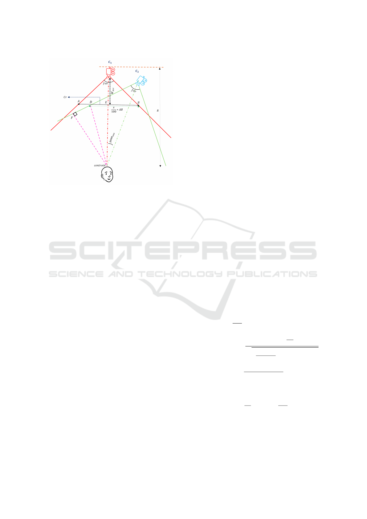
Figure 3: Derivation of step size of yaw in 2D.
need not be constrained on FoV if C is defined as pro-
posed.
3.3 Optimization of Camera Search
Space
To geometrically optimize C, we solve for an arrange-
ment of cameras in which adjacent cameras share a
minimum degree of overlap between their coverage.
This criterion is driven by the need for a minimum of
2 views for triangulation. Spherical placement is the
optimal placement which we show empirically in the
following sections.
We assume all the candidate cameras are static
perspective cameras with the same horizontal and ver-
tical FoV. The camera lens has a minimum and max-
imum working distance within which the scene can
be captured with adequate focus and resolution. The
scene captured by any one camera is a frustum of a
quadrilateral pyramid.
The cameras can be placed on the surface of a
3D sphere constructed around the centroid of the
control space (Q) which is denoted by centroid.
(X
C
j
,Y
C
j
,Z
C
j
,Yaw
C
j
,Pitch
C
j
) of C
j
are worked out
given the sphere’s radius (R), the field of view of C
j
,
and the overlap of coverage desired between adjacent
cameras. Given the geometric structure of frustum,
ensuring that the head is covered at the nearest depth
(Z
Q
i
) within the control space will automatically guar-
antee coverage at Z > Z
Q
i
. The critical region (Cr) is
the width of the volume that needs to be covered by
a camera and is dependent on the use case. Let us
consider an x% overlap in the critical region between
adjacent cameras. This means the overlap at greater
depths within the control space will be > x%. Re-
garding the amount of overlap, as shown in fig. 2, C
1
and C
2
can cover the fiducial points on the left side of
the head, while C
2
and C
3
can cover the right. A 50%
overlap would have sufficed if the head were static.
However, to ensure complete coverage of the fidu-
cial points throughout the control space, we opt for an
overlap greater than 50%. This approach guarantees
ample options for the BIP to select from in the cam-
era search space. We determine the radius R based
on the largest sphere that can fit within the 3D en-
vironment. A C derived from Cr and R evades the
need of explicitly constraining OCP on FoV. Consid-
ering all these factors, we derive the pose
step
in a di-
mension at which the cameras should be positioned
on the sphere, and the same method can be applied
to calculate the steps in other dimensions as well.
The pose
step
(yaw
step
, pitch
step
) can derive yaw
C
i
and
pitch
C
i
of cameras. X
C
i
,Y
C
i
,Z
C
i
can be easily indexed
as a point on the sphere using yaw
C
i
and pitch
C
i
. Al-
gorithm for building spherical camera search space
using calculated steps of yaw
step
and pitch
step
is given
in 2.
The coverage overlap computation at the critical
region of control space is done in 2D for simplifica-
tion. A sample derivation of pose
step
required for R
radius, x% overlap on (Cr) in 2D in shown in fig. 3.
In fig 3, we solve for ∠C
1
OC
2
. Here, the criti-
cal region (Cr) that must always be covered by C
1
, is
highlighted by AB. The minimum working distance
(W
dist
) of camera C
1
is given by C
1
E and can be de-
rived based on Cr and f ov of C
1
. In 2D, the coverage
overlap between the cameras C
1
and C
2
is represented
by BD. The step size ∠C
1
OC
2
is solved for by setting
BD to x % of AB which boils down to -
∠C
1
OC
2
= 90 −
f ov
2
− cos
−1




R · cos

f ov
2

r

(x−50)·Cr
100

2
+ (R −W
dist
)
2




− tan
−1

(x − 50) ·Cr
(R −W
dist
) · 100

(6)
where W
dist
is given as
W dist =
Cr
2
· tan(90 −
f ov
2
) (7)
Note that the critical region (Cr), radius R and f ov
are coupled to each other and are not free variables.
As (Cr) increases, R may have to be increased to ac-
commodate the more exhaustive coverage.
Optimal Camera Placement for 6D Head Pose Estimation
85

Figure 4: Camera Search Space: Uniform vs Spherical. To
cover the same region, the uniform placement requires more
cameras than the virtual placement.
3.3.1 Why a Spherical Placement?
When creating the camera search space for an
arbitrary-shaped target 3D environment, intuitively,
we may place the cameras all over the surface as
shown by the outer polygon in fig. 4, encapsulating
the region of interest. Naively placing cameras on the
surface or dividing the possible camera configuration
space into uniformly spaced grids may lead to redun-
dancy of cameras in visibility space and may not en-
sure sufficient camera options for the BIP.
The bigger the camera search space, the longer
the computation time for building the visibility con-
straints. However, a bigger camera space does not
necessarily ensure an optimal solution. This geomet-
ric placement of candidate cameras, derived from the
visibility requirements, ensures a relatively more op-
timal solution than the uniform placement.
3.3.2 Generalizability to a Bigger 3D
Environment
The camera solution derived from spherically placed
cameras is reusable. It can easily adapt to any larger
arbitrary 3D environment. A camera can be moved
along the line connecting the camera to the centroid,
which is also the camera’s optical axis in this sce-
nario. The camera’s depth can be scaled up spatially
(camera can be pushed back) from its original 3D lo-
cation as long as the face is captured at some min-
imum resolution needed for a good performance of
2D landmark detector. The concept has been quali-
tatively demonstrated with some examples and math-
ematical proof for the same is given in appendix 13.
We present the following reasons to justify that mov-
ing the cameras along their optical axis ensures max-
imum reusability-
1. The optical axis of all the cameras in the solution
intersect at the centroid, which is also the center
of the sphere. When the camera is scaled along
the optical axis:
Figure 5: Compensation of visibility on up-scaling of cam-
eras.
(a) There is no change in the head’s visibility lo-
cated at centroid. Only the size of the head in
the image changes, and hence it does not affect
the visibility of the fiducials.
(b) When the head is not at the centroid, the visibil-
ity is affected, but it is least compared to trans-
lating the camera in any other direction. In fig.
6 , camera C
1
, a part of the camera solution,
can see points P
1
, P
2
and P
3
. Pushing C
1
to
C
′
1
can still see all 3 points. Pushing C
1
to C
2
will favor the visibility of P
1
and P
2
, however,
will lose P
3
. In addition to losing the visibil-
ity of P
3
, such translations of cameras will have
a cascading effect on the remaining cameras in
the solution. Computing equivalent transforma-
tions/translation of remaining cameras to com-
pensate for the loss of visibility of fiducials is
non-trivial. It is as bad as solving the binary
integer program all over again. A generaliz-
able method, like ours, must preserve the con-
straints satisfied by the original camera network
as much as possible.
2. Moreover, a single camera’s coverage might be af-
fected by the upscaling along optical axis. How-
ever, combined coverage of the original solution
from all the cameras is maintained in the upscaled
solution. For example, in fig. 5, the left eye inner
corner was visible in C
1
which upon scaling C
′
1
is now unable to capture it due to obstruction by
nasian bridge. On the other hand, the same fidu-
cial was originally out of FoV of C
2
, and is now
captured by C
′
2
.
3.4 Approximate Visibility
Building visibility constraints for a Q
i
requires com-
puting Vis(∗,Q
i
,C
j
) with respect to all C
j
in C, which
is time-consuming and computationally intensive. We
propose that visibility need not be computed for
points at all depths and from all cameras. The visi-
ICINCO 2025 - 22nd International Conference on Informatics in Control, Automation and Robotics
86

Figure 6: Visibility preservation is maximal for a translation
along the camera’s line of sight.
bility flags of the fiducial points can be precomputed
on a wide range of head positions and orientations
from one camera and at one depth (Z
f ixed
), and looked
up while building visibility constraints with respect to
the other cameras on the fly.
Visibility is unaffected when P
′
k
= α ∗ P
k
, meaning
a fiducial P
k
is moved along the camera’s line of sight
by a scale of α. If any other point P
l
can be expressed
as a scaled version of P
k
, the visibility of P
l
will be the
same as that of P
k
. Readers may refer to the appendix
13 for proof.
Every 3D point can be represented as a scaled ver-
sion of a point at a fixed depth Z
f ixed
. Hence, the
visibility of control points need not be computed at
all depths, as long as we have the visibility flag of
a scaled version of P
k
at Z
f ixed
available. If the ex-
act match is unavailable in the visibility lookup ta-
ble LU T
vis
, the visibility flag of the nearest control
point is used. This approach can be used in cases
where a certain degree of approximation is acceptable
to trade off with the runtime computation. To reduce
the approximation, LUT
vis
must be populated with a
finer granularity and broader ranges of head positions
(X,Y ) and orientations (yaw, pitch, and roll).
A LUT
vis
is populated with visibility flags
for N
K
fiducials at (|yaw r anges| ∗ |pitch ranges| ∗
|roll ranges|) head orientations and (|X ranges| ∗
|Y ranges| head positions computed at Z = Z
f ixed
.
A step-by-step algorithm for obtaining (approximate)
visibility of P
k
from C
j
given a LU T
vis
is shown in
algorithm 1.
4 EVALUATION
To evaluate the effectiveness of our approach, we de-
fine the metrics as follows -
1. Conciseness(N
S
): The fewer cameras in the solu-
tion, the more concise the multi-view solution.
2. Test Visibility Metric(η): The control points that
failed to be captured by two or more cameras are
categorized as Failure. Test visibility is defined
as -
η = 1 −
Failure
N
test
Q
(8)
where N
test
Q
is the size of test control space.
3. Constraint Building Time (T
vis
) : Time complexity
for building visibility constraints is O(N
Q
∗ N
C
∗
N
K
) as there are N
Q
visibility constraints for each
of the N
K
fiducial points. Building each constraint
requires visibility computation from each of N
C
cameras.
4. Camera Exposure Rate (β): We define the cam-
era exposure rate of a fiducial point as the average
number of cameras in the multi-view solution that
can capture the fiducial point.
Algorithm 1: Algorithm depicting the proposed approxi-
mate visibility computation of P
k
from camera C
j
.
Input: Visibility Lookup
LUT
vis
[yaw ranges,
pitch ranges,rol l ranges,X ranges,Y ranges]
Control Point
P
k
: yaw
p
, pitch
p
,roll
p
,X
p
,Y
p
,Z
p
Camera C
j
: yaw
c
, pitch
c
,X
c
,Y
c
,Z
c
Depth Z
f ixed
Rotation matrix to euler angles : euler()
Euler angles to rotation matrix : rot mtx()
Output: Approximate visibility of P
k
wrt C
j
t
p
= [X
p
,Y
p
,Z
p
]
t
c
= [X
c
,Y
c
,Z
c
]
R
p
= rot mtx(yaw
p
, pitch
p
,roll
p
)
R
c
= rot mtx(yaw
c
, pitch
c
,0)
R
p,c
= R
p
.R
c
T
yaw
p,c
, pitch
p,c
,roll
p,c
= euler(R
p,c
)
t
p,c
= (t
p
− t
c
).R
c
X
p,c
,Y
p,c
,Z
p,c
= t
p,c
X
′
p,c
= (Z
f ixed
/Z
p,c
) ∗ X
p,c
Y
′
p,c
= (Z
f ixed
/Z
p,c
) ∗Y
p,c
yaw
′
= argmin
y
i
∈yaw ranges
|y
i
− yaw
p,c
|
pitch
′
= argmin
p
i
∈pitch ranges
|p
i
− pitch
p,c
|
roll
′
= argmin
r
i
∈roll ranges
|r
i
− roll
p,c
|
X
′
= arg min
X
i
∈X ranges
|X
i
− X
p,c
|
Y
′
= argmin
Y
i
∈Y ranges
|Y
i
−Y
p,c
|
vis = LUT
vis
[yaw
′
][pitch
′
][roll
′
][X
′
][Y
′
]
return vis;
The mathematical proof showing the correctness
of the proposed approximate visibility flags from pre-
computed visibility is given in the appendix 6.
Optimal Camera Placement for 6D Head Pose Estimation
87

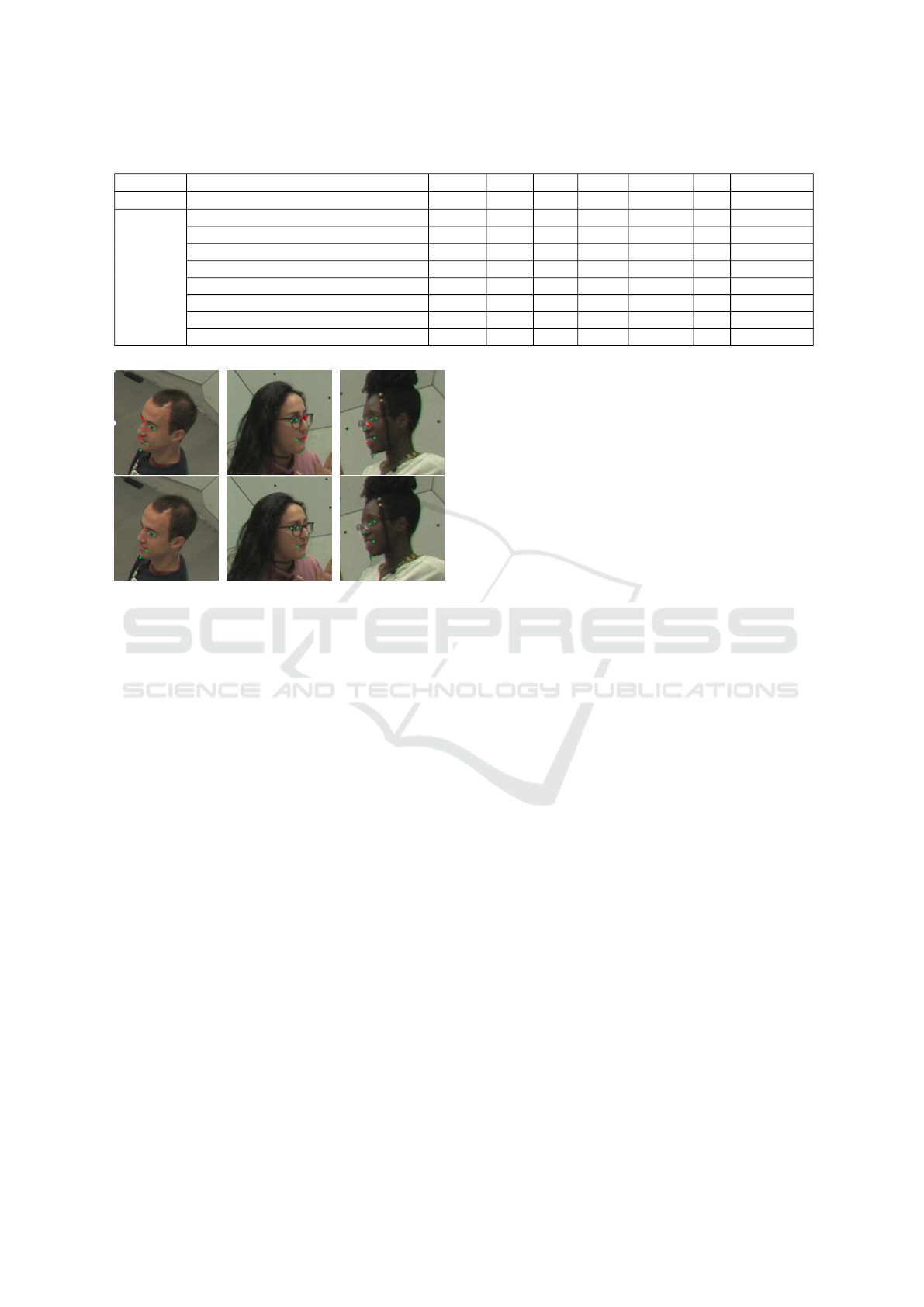
Table 1: Performance of experiments with different configurations of camera search space.
Configuration Radius N
C
N
S
↓ η ↑ Failure↓ β ↑ T
vis
(s/iter)↓
Baseline Uniform Placement of Camera - 5416 15 0.854 111529 3 133
Our
Method
Default 500 325 31 0.998 1113 11 12
Diagonal(20
◦
,20
◦
) 500 975 20 0.998 1320 8 27
Translational(100) 500 975 19 0.998 839 8 27
Diagonal & Translational(20
◦
,20
◦
,100) 500 1625 18 0.998 1247 7 40
Default 800 325 10 0.999 477 5 12
Diagonal(20
◦
,20
◦
) 800 975 9 0.999 195 5 27
Translational(200) 800 975 9 0.999 296 5 27
Diagonal & Translational(20
◦
,20
◦
,200) 800 1625 9 0.999 309 5 40
Figure 7: Example images from CMU Panoptic Dataset.
The first row shows visible fiducials according to the
dataset. The second row shows the visible fiducials accord-
ing to our algorithm. Non-visible(incorrect) fiducials are
colored red.
5 EXPERIMENTS
5.1 Visibility Algorithm
The head mesh model, FLAME[(Li et al., 2017)]
is used to model self-occlusion of fiducials. It has
N
v
= 5023 vertices and N
f
= 9976 triangles. We show
the precision of the visibility algorithm on a public
dataset, CMU Panoptic Dataset [(Joo et al., 2016)], a
multi-view dataset captured in a 3D environment with
31 HD cameras. It has 3D facial landmarks and cor-
responding visibility flags from all the cameras. We
compare the ground truth visibility flags of the fol-
lowing fiducials from the dataset with visibility com-
puted from our method- Left Eye Inner Corner, Left
Eye Outer Corner, Right Eye Inner Corner, Right Eye
Outer Corner, Left Mouth corner, Right Mouth cor-
ner, Nose Tip, Chin. fig. 7 shows the qualitative re-
sults.
5.2 Spherical Placement of Candidate
Cameras
Coordinate System: In our experiments, we have as-
sumed the X-axis to the right, Y-axis downwards, Z-
axis into the screen.
We solve the problem using a small control space
of size N
Q
= 768 and test the solution on a 3X finely
sampled control space of size N
test
Q
96000. The 6D
ranges of runtime control space and test control space
are defined in Table 2. As for fiducial points, we con-
strain OCP on the visibility of all the fiducials men-
tioned in section 5.1. We do not add FoV constraints
(eq. 4) as they are implicitly satisfied by all the can-
didate cameras. All experiments use an open-source
CBC solver[(Forrest et al., 2024)].
Baseline: Assuming the scene is set in a rectangular
room, we imitate the baseline by placing 5416 cam-
eras in uniform grids on the front and side walls, with
the person’s head directed towards the front wall.
Our Method: Camera search space is created as de-
scribed in section 3.3. In 6, the horizontal and verti-
cal f ov is set to 90
◦
,hence, yaw
step
= pitch
step
. We
present results for two radii: 500mm and 800mm. For
the experiments with R = 500mm, the Cr is set to
200mm with an overlap of x = 60%, resulting in a
pose
step
of 14.11
◦
. For the R = 800mm, the Cr is
set to 400mm with an overlap of x = 75%, yielding
pose
step
of 13.96
◦
. In both cases, the step sizes are
approximated to 15
◦
. As stated earlier, Cr,R and f ov
are interrelated, implying that the geometry in fig. 3
may change if the variables are geometrically incon-
sistent. For instance, targeting a Cr of 400mm with
radius of 500mm will modify the geometry of fig. 3
and in turn the eq. 6. Experiments with optimized
search space are performed in 4 different augmenta-
tion settings -
1. Default Configuration - Placing the cameras over
the sphere at steps of 15
◦
yaw and pitch.
2. Diagonal Augmentation (aug
yaw
,aug
pitch
) -
(a) Default Configuration
ICINCO 2025 - 22nd International Conference on Informatics in Control, Automation and Robotics
88

(b) 2 additional cameras oriented at
aug
yaw
,aug
pitch
• yaw
C
j
+ aug
yaw
, pitch
C
j
+ aug
pitch
• yaw
C
j
− aug
yaw
, pitch
C
j
− aug
pitch
3. Translational Augmentation (aug
trans
) -
(a) Default Configuration
(b) 2 additional cameras translated at
• X
C
j
+ aug
trans
• X
C
j
− aug
trans
4. Diagonal & Translational Augmentation
(aug
yaw
,aug
pitch
,aug
trans
) -
(a) Default Configuration
(b) 2 additional cameras rotated and translated at
• yaw
C
j
+ aug
yaw
, pitch
C
j
+ aug
pitch
• yaw
C
j
− aug
yaw
, pitch
C
j
− aug
pitch
• X
C
j
+ aug
trans
• Y
C
j
− aug
trans
In Setting 2, the default configuration is enhanced
by orienting the cameras diagonally at specific angles
from their original poses. In Setting 3, the default
setup is enhanced by cameras translated along a spec-
ified dimension. These augmentations aim to provide
BIP with more options, if needed. The results from
these augmented settings closely resemble those of
the default configuration, highlighting the effective-
ness of our approach. These augmentations represent
a trade-off between the conciseness of the solution
and the computational complexity of the search space,
allowing users to choose based on their specific use
case.
Our extensive experiments demonstrate that the
multi-view solution achieved through optimized ini-
tialization of the camera search space outperforms
the solution obtained from uniform camera placement
across all test metrics. The results in Table 1 indi-
cate that our method, with or without augmentation,
consistently achieves a high test visibility score (over
99%) while utilizing a much smaller camera search
space than the baseline.
A more concise camera search space also leads to
significantly reduced execution times compared to the
baseline. A low test visibility score is associated with
a poor-quality solution as it comes with a higher fail-
ure rate at intermediate control points. Although re-
sults from some of our experiments are not as com-
pact as those of the baseline solution, such as ones
with R = 500mm, solutions are still more desirable
due to their higher η, better β, and lower T
vis
.
Our best outcome, featuring a Diagonal (20, 20)
configuration with R = 800mm, is visualized in fig. 8.
The camera solution offers ≈ 14.5% increment on η
with 6 lesser cameras than the baseline solution. On
average, our method achieves a β of 5 or higher, com-
pared to the baseline score of 3.
Table 2: Range of runtime and test control space.
Dimension min max runtime step test step
yaw -90 60 30 10
pitch -60 30 30 10
roll -60 30 30 10
X 0 200 200 50
Y -400 -200 200 50
Z 300 500 200 50
5.3 Generalizability of Camera Solution
To simulate fitting to an arbitrary-shaped 3D environ-
ment, we upscale the cameras from the existing so-
lution by random factors. As seen in Table 3, the
count of test control points failing to be tracked by
the environment-adapted solution (Failure
adapted
) is
less than or equal to failures of the original solution
(Failure
original
).
The experimental results in Table 1 and 3 high-
light the optimality of spherical placement strategy
and adaptability of the solutions, respectively.
Table 3: Performance of environment-adapted camera solu-
tion vs original solution.
Failure
original
↓ Scale Range Failure
adapted
↓
1113 1.5-2.0 0
1247 1.0-1.5 121
195 1.2 - 1.6 61
5.4 Camera Placement from Proposed
Approximated Visibility
To test our proposed approximated visibility as ex-
plained in 3.4, we experiment with 2 LUT
vis
of dif-
ferent granularities. Both the lookups are populated
with visibility flags of the required fiducials in the
range of: yaw [−180
◦
,180
◦
], pitch [−90
◦
,90
◦
], roll
[−180
◦
,180
◦
] at steps of 10
◦
, 10
◦
, 10
◦
, respectively,
and X and Y in range of [−700,500]mm, much big-
ger than runtime Q [2]. The visibility for the above
range of poses is calculated at Z
f ixed
= 500mm. The
lookup C-50 has visibility flags stored at spatial gran-
ularity (X and Y ) of 50mm, C-25 at 25mm. As can
be noticed from the results in Table 4, both solutions
include a much smaller number of cameras but more
invisible test control points than the original solution.
The C-50 configuration exhibits greater sparsity in the
X and Y dimensions than the C-25 configuration, re-
sulting in the solver using less precise visibility flags
than those used in the C-25 configuration. Compu-
tationally, the lookup creation can be treated as pre-
Optimal Camera Placement for 6D Head Pose Estimation
89

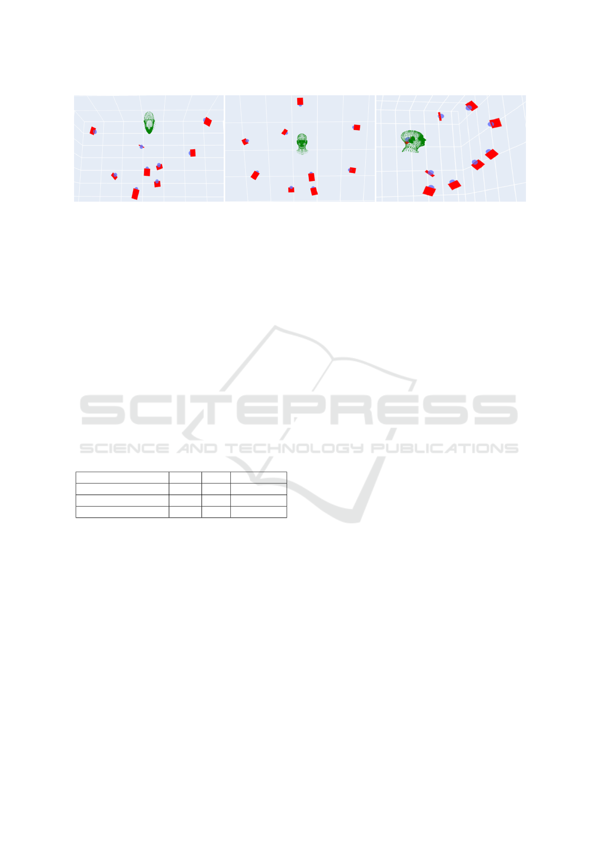
Figure 8: A sample camera solution from our method a) Top View, b) Front View, c) Side View.
processing and utilized for multiple integer programs
constrained on various definitions of Q. The trade-off
between the performance of a multi-view system and
its conciseness highly depends on the nature of the
application.
6 CONCLUSION
This work revisits the OCP for 6D head pose esti-
mation where we propose an optimized initialization
of camera search space and redefine visibility of 3D
points. Furthermore, as an alternative to the computa-
tionally intensive task of calculating visibility for all
fiducials from every camera, we introduce an algo-
rithm for approximate visibility computation. As a
future work, the solution can be extended to be de-
rived from a candidate set of varied focal lengths and
PTZ cameras.
Table 4: Performance with Approximated Visibility.
Lookup Configuration η ↑ N
S
↓ t
vis
(s/iter) ↓
Original 0.998 18 27
C-25 0.878 10 0.07
C-50 0.716 10 0.07
REFERENCES
Bettahar, H., Morsly, Y., and Djouadi, M. S. (2014).
Optimal camera placement based resolution re-
quirements for surveillance applications. In 2014
11th International Conference on Informatics in
Control, Automation and Robotics (ICINCO),
volume 01, pages 252–258.
Chv
´
atal, V. (1975). A combinatorial theorem in plane
geometry. Journal of Combinatorial Theory, Se-
ries B, 18(1):39–41.
Forrest, J., Ralphs, T., Vigerske, S., Santos, H. G.,
Forrest, J., Hafer, L., Kristjansson, B., jpfasano,
EdwinStraver, Jan-Willem, Lubin, M., rlougee,
a andre, jpgoncal1, Brito, S., h-i gassmann,
Cristina, Saltzman, M., tosttost, Pitrus, B., MAT-
SUSHIMA, F., Vossler, P., SWGY, R. ., and to st
(2024). coin-or/cbc: Release releases/2.10.12.
H
¨
orster, E. and Lienhart, R. (2006). On the opti-
mal placement of multiple visual sensors. In
Proceedings of the 4th ACM International Work-
shop on Video Surveillance and Sensor Net-
works, VSSN ’06, page 111–120, New York,
NY, USA. Association for Computing Machin-
ery.
Joo, H., Simon, T., Li, X., Liu, H., Tan, L., Gui,
L., Banerjee, S., Godisart, T., Nabbe, B. C.,
Matthews, I. A., Kanade, T., Nobuhara, S., and
Sheikh, Y. (2016). Panoptic studio: A massively
multiview system for social interaction capture.
CoRR, abs/1612.03153.
Li, T., Bolkart, T., Black, M. J., Li, H., and Romero,
J. (2017). Learning a model of facial shape and
expression from 4d scans. ACM Trans. Graph.,
36(6).
Liu, J., Sridharan, S., Fookes, C., and Wark, T.
(2014). Optimal camera planning under versa-
tile user constraints in multi-camera image pro-
cessing systems. IEEE Transactions on Image
Processing, 23(1):171–184.
O’Rourke, J. (1993). On the rectilinear art gallery
problem. Computational Geometry, 3(1):53–58.
Puligandla, V. A. and Lon
ˇ
cari
´
c, S. (2022). A mul-
tiresolution approach for large real-world cam-
era placement optimization problems. IEEE Ac-
cess, 10:61601–61616.
Zhang, H., Eastwood, J., Isa, M., Sims-Waterhouse,
D., Leach, R., and Piano, S. (2021). Optimi-
sation of camera positions for optical coordi-
nate measurement based on visible point anal-
ysis. Precision Engineering, 67:178–188.
Zhang, X., Chen, X., Alarcon-Herrera, J. L., and
Fang, Y. (2015). 3-d model-based multi-camera
deployment: A recursive convex optimization
approach. IEEE/ASME Transactions on Mecha-
tronics, 20(6):3157–3169.
ICINCO 2025 - 22nd International Conference on Informatics in Control, Automation and Robotics
90

Zhao, J., Cheung, S.-C., and Nguyen, T. (2008). Op-
timal camera network configurations for visual
tagging. IEEE Journal of Selected Topics in Sig-
nal Processing, 2(4):464–479.
APPENDIX
Translating the head without any change in rotation
changes the view of the object in the camera, affect-
ing the visibility of the fiducial points. Similarly, ro-
tating the object without translating it also affects the
visibility of the fiducials. However, there is a special
case of translating the object, so the visibility is un-
affected. This happens when the object is translated
along the camera’s line of sight. Given an image I
of a head translated at a 3D location H = [H
x
,H
y
,H
z
]
in camera C
j
, when moved along the camera’s line of
sight to the new position H
′
= α ∗ H, the correspond-
ing image I
′
=
1
α
∗ I about the 2D projection of H in
I.
For proof, let the camera projection matrix and a
perspective projection of point X rotated and trans-
lated by R and T, respectively, be given as
K =


f
x
0 c
x
0 f
y
c
y
0 0 1


, pro j(X) = K[RX + T ] (9)
For simplicity, let us assume the translation of the
head is done with respect to a central facial point
which we address by head center H. In action, all
the points in the head are rotated first and then trans-
lated. Hence, in neutral pose, the head center will
be at [0,0,0], i.e., the origin of the coordinate sys-
tem. Any amount of rotation applied to the head cen-
tre at [0, 0, 0] will keep the 3D location of the head
unchanged at [0,0,0]. Hence,
pro j(X) = K[RX + H] = pro j(H) (10)
when X is the head center in neutral pose.
Proof 1 : When H
′
→ α ∗ H, pro j(H) = pro j(H
′
)
Solving LHS,
pro j(H) = K[H] =
"
f
x
∗
H
x
H
z
+ c
x
f
y
∗
H
y
H
z
+ c
y
#
(11)
Solving RHS,
pro j(H
′
) = K[α ∗ H] =
"
f
x
∗
α∗H
x
α∗H
z
+ c
x
f
y
∗
α∗H
y
α∗H
z
+ c
y
#
(12)
Proof 2 : When H
′
→ α ∗ H, I
′
→
1
α
∗ I
Let the facial landmarks be denoted by P =
[P
1
,P
2
,...,P
N
k
] where P
i
= [P
x
,P
y
,P
z
] (we will work
with one sample fiducial point, for simplicity denoted
by P). Upon scaling, H
′
= α∗H, P
′
= P +(α−1)∗H
Knowing that an image is a set of 2D points, we
consider the distance between any two known 2D
points to compute the equivalent transformation to be
applied to the image.
Proof boils down to,


pro j(H
′
) − pro j(P
′
)


2
=
1
α
·
∥
pro j(H) − pro j(P)
∥
2
(13)
Solving RHS,
=
1
α
·
s

f
x
·
H
x
H
z
+ c
x

−

f
x
·
P
x
P
z
+ c
x

2
+

f
y
·
H
y
H
z
+ c
y

−

f
y
·
P
y
P
z
+ c
y

2
=
1
α
·
s
f
2
x
·

H
x
H
z
−
P
x
P
z

2
+ f
2
y
·

H
y
H
z
−
P
y
P
z

2
(14)
Solving LHS,
pro j(P
′
) = pro j(P + H
′
− H)
=
"
f
x
(P
x
+(α−1)H
x
)+c
x
(P
z
+(α−1)H
z
)
P
z
+(α−1)H
z
f
y
(P
y
+(α−1)H
y
)+c
y
(P
z
+(α−1)H
z
)
P
z
+(α−1)H
z
#
(15)
To simplify the above equation, we make a realistic
assumption of H
z
≈ P
z
, meaning the facial landmarks
are approximately at the same depth as the head
center H. With this assumption, LHS becomes -
=
s

f
x
·
H
x
H
z
+ c
x
− f
x
·
(P
x
+ (α − 1)H
x
)
αH
z
+ c
x

2
+

f
y
·
H
y
H
z
+ c
y
− f
y
·
(P
y
+ (α − 1)H
y
)
αH
z
+ c
y

2
=
s

f
x
·
H
x
H
z
− f
x
·
(P
x
+ (α − 1)H
x
)
αH
z

2
+

f
y
·
H
y
H
z
− f
y
·
(P
y
+ (α − 1)H
y
)
αH
z

2
=
s
f
2
x
·

H
x
H
z
−
P
x
P
z

2
+ f
2
y
·

H
y
H
z
−
P
y
P
z

2
(16)
Optimal Camera Placement for 6D Head Pose Estimation
91

Algorithm 2: Spherical Placement of Cameras.
Input: yaw
step
, pitch
step
, R, centroid
Output: Camera Search Space C
centroid
X
,centroid
Y
,centroid
Z
= centroid;
C = {};
yaw = 0
◦
;
pitch = 0
◦
;
while yaw ≤ 360
◦
do
while pitch ≤ 360
◦
do
yaw
C
j
, pitch
C
j
= −yaw,−pitch
X
C
j
=
centroid
X
+ R · cos(pitch) · sin(yaw)
Y
C
j
= centroid
Y
− R · sin(pitch)
Z
C
j
=
centroid
Z
− R · cos(pitch) · cos(yaw)
C
j
= (X
C
j
,Y
C
j
,Z
C
j
,yaw
C
j
, pitch
C
j
)
Add C
j
in C
yaw ← yaw + yaw
step
pitch ← pitch + pitch
step
end
end
return C;
ICINCO 2025 - 22nd International Conference on Informatics in Control, Automation and Robotics
92