Verifying Positivity of Piecewise Quadratic Lyapunov Functions*

Sigurdur Hafstein

and Eggert Hafsteinsson

University of Iceland, Faculty of Physical Sciences, Dunhagi 5, 107 Reykjavik, Iceland

Keywords:

Lyapunov Function, Piecewise Quadratic, Numerical Algorithm, Switched Systems, Cone-Wise Linear

Systems.

Abstract:

Continuous, piecewise quadratic (CPQ) Lyapunov functions are frequently used to assert stability for switched,

cone-wise linear systems. It is advantageous to construct such Lyapunov functions in two steps: ﬁrst a function

is parameterized that is decreasing along all system trajectories, then it is veriﬁed whether this function is

positive deﬁnite. Usually these steps have been performed using linear matrix inequalities (LMIs), but recently

a linear programming (LP) approach for the ﬁrst step has been suggested. In this paper we present a new

algorithm to verify the positivity of CPQ Lyapunov function candidates, parameterized either with LMIs or

LP. Further, we prove that the algorithm is non-conservative and will always be able to either assert positive

deﬁniteness of a CPQ Lyapunov function candidate or ﬁnd a point where it is negative.

1 INTRODUCTION

Switched, cone-wise linear systems have received

much interest in the control engineering community,

in particular since the seminal works of Mikael Jo-

hansson and Anders Rantzer (Johansson and Rantzer,

1998; Johansson, 1999). For these systems, the sta-

bility of the origin has been, inter alia, asserted by us-

ing continuous and piecewise afﬁne (CPA) Lyapunov

functions, see e.g. (Andersen et al., 2023b; Ander-

sen et al., 2023a), or by using continuous and piece-

wise quadratic (CPQ) Lyapunov functions as in the

works of Johansson and Rantzer. Such systems have,

for example, been successfully used to study hybrid

integrator-gain systems (HIGS), see e.g. (van den Ei-

jnden et al., 2020; Deenen et al., 2021; van den Eijn-

den et al., 2022).

Recently an algorithm different to the usual lin-

ear matrix inequality (LMI) approach for the com-

putation of CPQ Lyapunov functions was presented,

where linear programming (LP) is used instead of

semi-deﬁnite optimization to parameterize CPQ Lya-

punov functions, see (Palacios Roman et al., 2024;

Andersen et al., 2024). Just as in the LMI approach,

it is advantageous to construct the CPQ Lyapunov

function in two steps; see Section 4.8 in (Johansson,

1999). First, a CPQ real-valued function V from the

https://orcid.org/0000-0003-0073-2765

∗

This work was supported in part by the Icelandic Re-

search Fund under Grant 228725-051.

state-space is parameterized, that is decreasing along

all system trajectories; this function is referred to as

Lyapunov function candidate. In a second step it is

veriﬁed whether V is positive deﬁnite or not. If V

is positive deﬁnite, i.e. V (0

0) = 0 and V(x) > 0 for

all x ∈ R

\ {0

0}, then V is a Lyapunov function for

the system and the origin is asymptotically stable. If

there exists an x ∈ R

\ {0

0} such that V (x) < 0, then

the origin is unstable. Both of these properties follow

from the fact that V is decreasing along all system tra-

jectories. In more detail: If V is positive deﬁnite, then

all solution trajectories must approach the minimum

at the origin. If there is an x ∈ R

\ {0

0} such that

V (x) < 0, then V (ax) < 0 for all a > 0, and solutions

starting at a point ax must approach inﬁnity, where the

values of V are lower. It follows that it is impossible

that V takes on negative values if the origin is asymp-

totically stable. Further, the third possibility, i.e. that

V (x) ≥ 0 for all x ∈ R

and there is an y ∈ R

differ-

ent to the origin such that V (y) = 0, is impossible; see

Theorem 1.

Hence, dividing the algorithm into two steps is

not only computationally more efﬁcient, but asymp-

totic stability of the origin will be asserted if it is

asymptotically stable, and as an added bonus, insta-

bility can be asserted for instable systems. The main

contribution of this paper is the presentation of a new

algorithm to verify the positivity of CPQ Lyapunov

function candidates parameterized with the method

from (Palacios Roman et al., 2024; Andersen et al.,

Hafstein, S. and Hafsteinsson, E.

Verifying Positivity of Piecewise Quadratic Lyapunov Functions.

DOI: 10.5220/0013713600003982

Paper published under CC license (CC BY-NC-ND 4.0)

In Proceedings of the 22nd International Conference on Informatics in Control, Automation and Robotics (ICINCO 2025) - Volume 1, pages 435-444

ISBN: 978-989-758-770-2; ISSN: 2184-2809

435

2024) or by LMIs. We prove in Theorem 11 that this

new method is non-conservative. Note that our new

algorithm is computationally more efﬁcient than the

LMI approach from (Johansson, 1999), discussed in

Section 2.4, which additionally introduces some con-

servatism; see e.g. (Scherer, 2006) for various LMI

relaxation methods used in control theory. Further,

our approach can be used to verify positivity for more

general functions than piecewise quadratic. Compar-

ison with more recent LMI approaches presented in

(Kruszewski et al., 2009; Sala and Arino, 2007; Gon-

zaleza et al., 2017), which are sufﬁcient and asymp-

totically necessary, will be the subject of a subsequent

publication.

2 CPQ LYAPUNOV FUNCTIONS

In this paper we consider switched, cone-wise linear

systems and CPQ Lyapunov functions that are posi-

tively homogeneous of order two. For this it is ad-

vantageous to ﬁrst consider triangulations of a neigh-

borhood of the origin of a speciﬁc type and then ex-

tend these triangulations to a conical subdivision of

the whole state-space R

. Hence, we ﬁrst deﬁne trian-

gulations suitable for our application, before we dis-

cuss conical subdivisions, our class of systems, and

CPQ Lyapunov functions.

2.1 Triangulations

A triangulation T of a set D

⊂ R

is a set of

n-simplices T := {S

: ν ∈ I}, such that D

ν∈I

; I is an index set. Recall that an n-simplex

is deﬁned as

:=co{x

,...,x

}

(

x ∈ R

: x =

∑

i=0

,λ

≥ 0,

∑

i=0

= 1

)

where the vectors x

∈ R

are called the vertices

of S

and are assumed to be afﬁnely independent,

i.e. the vectors x

− x

, i = 1,2,...,n are linearly in-

dependent. For our purposes, we additionally require

that the triangulation T is shape-regular, i.e., every

two different simplices S

∈ T either intersect in

a common lower-dimensional face or do not intersect

at all. This means that if S

∩S

̸=

0, then S

∩S

a k-simplex, 0 ≤ k < n, whose vertices are the vertices

common to S

and S

For our speciﬁc application we further demand

that x

= 0

0 for all S

∈ T and that D

is a neigh-

borhood of the origin 0

0 ∈ R

An efﬁcient implementation of a triangulation

that satisﬁes these requirements is the triangular fan

std

K,fan

, K ∈ N := {1,2,...}, discussed in (Hafstein,

2019) where a formula for the vertices x

is given.

In the following we write T

for T

std

K,fan

. The vertex

set of the triangulation T

, i.e. the set of all vertices

of all simplices, is

0} ∪

{

z ∈ Z

∥

∞

= K

}

where the scaling parameter K ∈ N determines the

ﬁneness of the triangulation around zero. The num-

ber of simplices in the triangulation T

is given by

the formula 2

· K

n−1

· n!.

For computations it is usually better to map the

vertices T

with the mapping F : R

→ R

, F(0

0) = 0

and F(x) =

∥x∥

∞

∥x∥

x. The resulting triangulation is de-

noted T

and the set D

is approximately spheri-

cally symmetric, see Figures 1 and 2.

For proving theorems, it is often convenient to

scale down all the vertices of T

by the factor K

−1

The resulting triangulation is denoted K

−1

and all

its non-zero vertices are at the boundary of the unit

hypercube [−1,1]

and for any two different non-

zero vertices x,y of a simplex S

∈ K

−1

we have

∥x −y∥

∞

= K

−1

For a ﬁxed K ∈ N, all the triangulations T

, T

and K

−1

give the same conical subdivision of the

state-space R

discussed in the next section.

2.2 Conical Subdivision of the

State-Space

Given a triangulation T as in the last section, one

can deﬁne a corresponding conical subdivision of the

state-space through

:= {x ∈ R

: cx ∈ S

for some c > 0}

for every S

∈ T . Since S

= co{x

,...,x

} it is

easy to see that

= cone{x

,...,x

}

(

∑

i=1

: λ

≥ 0

)

Hence, every x ∈ C

has a unique set of numbers

,λ

,...,λ

≥ 0 such that x =

∑

i=1

because the

are linearly independent; recall that x

= 0

0. Since

T is a triangulation of a neighborhood of the origin

, the set-theoretic union of all C

is equal to R

2.3 Switched Linear Systems and CPQ

Lyapunov Functions

We consider systems of the form

x(t) = A

s(t)

x(t), A

∈ R

n×n

for j ∈ {1,2,...,M},

ICINCO 2025 - 22nd International Conference on Informatics in Control, Automation and Robotics

436

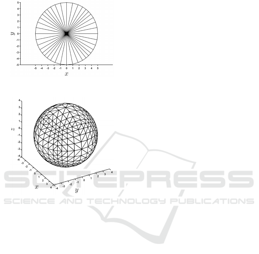
Figure 1: The triangulation T

in two dimensions and with

K = 5.

Figure 2: The triangulation T

in three dimensions and

with K = 4. Note that every simplex in T

is a tetrahedron

with zero as a vertex, together with three other vertexes at

the boundary of a sphere centered at the origin and with ra-

dius K.

where s : [0,∞) → {1,2,...,M}, M ∈ N, is a

right-continuous, piecewise constant function, called

switching signal, with a only a ﬁnite number of dis-

continuity points, called switching times, on any ﬁ-

nite time interval. The switching signal can either

be arbitrary, in which case the systems is said to be

arbitrary switched, or one can introduce restrictions

in the form σ(t) = j only if x(t) ∈ F

, where the

,...,F

⊂ R

are closed simplicial cones with

the apex at the origin, similar to the C

s above, ful-

ﬁlling that the

j=1

= R

and the intersection of

the interiors F

◦

and F

◦

of two different cones F

and

is empty. In the latter case the system is said to

have state-dependent switching; see (Palacios Roman

et al., 2024) for more details.

The solutions to arbitrary switched systems

are understood in the sense of Carathéodory, see

e.g. (Walter, 1998), and the solutions to systems with

state-dependent switching are understood in the sense

of Filippov, see (Filippov, 1988) or e.g. (Camlibel and

Pang, 2006) for cone-wise linear systems, which takes

care of sliding modes. For both arbitrary switched

systems and systems with state-dependent switching,

the origin is said to be globally uniformly exponen-

tially stable (GUES) if there exist constants c ≥ 1,

λ > 0 such that all solutions fulﬁll

∥x(t)∥

≤ ce

−λt

∥x(0)∥

for all t ≥ 0.

In both cases the GUES of the origin can be as-

serted with the existence of a CPQ Lyapunov function

fulﬁlling: Let {C

}

ν∈I

be a conical subdivision of the

state-space as in Section 2.2 and assume V : R

→ R

is a continuous function such that for, w.l.o.g. sym-

metric, matrices P

∈ R

n×n

we have

V (x) = x

x if x ∈ C

. (1)

Assume that the matrices P

∈ R

n×n

fulﬁll for

some constants c

> 0, that for all ν ∈ I and

all j ∈ {1,2,...,M} we have

∥x∥

≤ x

x ≤ c

∥x∥

, ∀x ∈ C

, (2)

+ P

)x ≤ −c

∥x∥

, ∀x ∈ C

∩ F

, (3)

where in (3) we set F

:= R

for all j in the case of

arbitrary switched systems.

We emphasize: if the conditions (2) and (3) are

fulﬁlled for the arbitrary switched system or the sys-

tem with state-dependent switching, the function V is

called a CPQ Lyapunov function for the system and

the origin is GUES; see e.g. Theorems 3 and 5 in

(Palacios Roman et al., 2024).

2.4 Computing CPQ Lyapunov

Functions

Both the LMI method from (Johansson and Rantzer,

1998; Johansson, 1999) and the LP method from

(Palacios Roman et al., 2024; Andersen et al., 2024)

parameterize a CPQ Lyapunov function candidate of

the form (1) fulﬁlling the conditions (3). The condi-

tions (2) are then veriﬁed a posteriori for the candidate

using the LMI:

For every ν ∈ I ﬁnd a symmetric matrix U

∈ R

n×n

with entries [U

]

i j

≥ 0 such that

− (X

−1

)

−1

⪰ 0, (4)

where ⪰ 0 means that the matrix on the left-hand-side

is symmetric and positive deﬁnite and



... x



∈ R

n×n

has the non-zero vertices of S

as its columns.

Since for every x ∈ C

there are unique λ

λ =

Verifying Positivity of Piecewise Quadratic Lyapunov Functions

437

(λ

,λ

,...,λ

)

, λ

≥ 0, such that x =

∑

i=1

, the

condition (4) implies for every such x ∈ C

that

0 ≤ x

− (X

−1

)

−1

)x (5)

= x

x −λ

Uλ

≤ x

The fact that V fulﬁlls the constraints 2 now easily fol-

lows from the fact that V is continuous, homogeneous

of order two, and that V (x) = 0 for x ̸= 0

0 is impossi-

ble if V (x) ≥ 0 for all x ∈ R

by the next theorem; see

also Section 3.2.

Theorem 1. Assume V is of the form (1) and fulﬁlls

the conditions (3). If V (x) ≥ 0 for all x ̸= 0

0, then

V (x) > 0 for all x ̸= 0

Proof. Let V fulﬁll the assumptions of the theorem

and assume V(ξ

ξ) = 0, ξ

ξ ̸= 0

0, and consider a solu-

tion x(t) starting at x(0) = ξ

ξ for an arbitrary switched

system. Let h > 0 be so small that x(t) ̸= 0

0 for all

0 ≤ t ≤ h, which is possible because x(t) is con-

tinuous, and so small that no switching occurs on

the interval [0,h]. Then for appropriate ν ∈ I and

j ∈ {1,2,...,M} we have

V (x(h)) = V (x(h)) −V (x(0)) =

V (x(t))dt

x(t)

+ P

)x(t)dt

≤ −c

∥x(t)∥

dt < 0 (6)

which contradicts V (x) ≥ 0 for all x ̸= 0

For systems with state-dependent switching this

follows similarly, but by the Fundamental Theorem of

Calculus for Lebesgue Integrals, see e.g. Chapter III,

Section 10 in (Walter, 1998). For Filippov solutions

we have

x(t) =

∑

j=1

(t)A

x(t),

∑

j=1

(t) = 1, a.e.,

for some non-negative functions λ

and since a.e.

V (x(t)) =

x(t)P

x(t) + x(t)

x(t)

∑

j=1

(t)x(t)

+ P

)x(t)

≤ −c

∥x(t)∥

we can conclude, similarly as in (6), that V (x(t)) < 0

for small enough t > 0, in contradiction to V (x) ≥ 0

for all x ̸= 0

Although the LMIs conditions (4) are sufﬁcient to

assert the conditions (2) for a CPQ Lyapunov func-

tion, they are not necessary. In the following section

we propose a different method that is both sufﬁcient

and necessary, and, as an added bonus, computation-

ally less demanding.

Remark 2. Note that the condition x

x ≥ 0 for all

x ∈ C

in (5) is nothing else than the condition of

copositivity of the matrix X

, i.e.

λ ≥ 0 for all λ

λ ∈ R

:= [0,∞)

This problem of deciding whether a matrix is coposi-

tive is known to be co-NP-complete; for more details

on copositive matrices see e.g. (Ikramov and Savel-

eva, 2000).

3 VERIFICATION OF

POSITIVITY

We start by discussing in general how the positivity of

a function deﬁned on a simplex can be veriﬁed. The

following lemma, proved as Lemma 4.16 in (Marinós-

son, 2002) using Taylor-expansions, is fundamental

for our approach:

Lemma 3. On an m-simplex S :=

co{x

,...,x

} ⊂ R

, m ≤ n, we have for a

function g ∈ C

(U), U ⊂ R

open neighbor-

hood of S, and every x =

∑

i=0

∈ S and any

d ∈ {0,1,. . . , n}, that



∑

i=0

) −

∑

i=0

g(x

)



≤

∑

i=0

, (7)

where

≥

∑

r,s=1

|[x

− x

]

|(|[x − x

]

| + |[x

− x

]

|),(8)

[y]

is the ith component of the vector y and

:= max

x∈S



∂

∂x

(x)



□

This lemma can be used to rigorously verify com-

putationally whether g(x) ≥ 0 on an m-simplex S :=

co{x

,...,x

} ⊂ R

, m ≤ n.

Test for Positivity 4. The test consist of the three fol-

lowing steps:

1. If g(x

) < 0 for some i ∈ {0, 1,...,m} then clearly

g(x) ≥ 0 for every x ∈ S does not hold true.

2. If

g(x

) − E

≥ 0 for i = 0,1,...,m, (9)

ICINCO 2025 - 22nd International Conference on Informatics in Control, Automation and Robotics

438

then, because

g(x) = g(x) −

∑

i=0

g(x

) +

∑

i=0

g(x

)

≥

∑

i=0

g(x

) − |g(x) −

∑

i=0

g(x

≥

∑

i=0

(g(x

) − E

) ≥ 0,

we have g(x) ≥ 0 for every x ∈ S.

3. If neither of the criteria above hold true, i.e. if

g(x

) ≥ 0 for all i = 0,1,...,m but there is an i ∈

{0,1,...,m} such that g(x

)−E

< 0, then the test

is inconclusive.

In the inconclusive case one can subdivide the

simplex S into smaller m-simplices and verify

whether g(x) ≥ 0 on these smaller simplices or not

with the same method. If we can guaranty that the

bounds E

s approach zero as the simplices get smaller

and smaller, this will indeed give us an algorithm that

asserts computationally that g(x) ≥ 0 for all x ∈ S

if min

x∈S

g(x) > 0. Further, if the vertices of the

ever further subdivided simplices build a dense set in

S, the method will also deliver a point x ∈ S with

g(x) < 0 if min

x∈S

g(x) < 0. Both these conditions

are easy to guaranty if the diameter of the simplices

converges to zero as we keep on subdividing the sim-

plices; we prove this in Corollary 8 and Lemma 10.

3.1 Some Notes on the Bounds E

For the term |[x − x

]

| in (8) we can use

max

j∈{0,1,...,m}

|[x

− x

]

| as an upper bound, which

is independent of x, because x =

∑

j=0

and



∑

j=0

− x



∑

j=0

− x

]



(10)

≤

∑

j=0



− x

]



≤ max

j∈{0,1,...,m}

|[x

− x

]

Hence, max

j∈{0,1,...,m}

|[x

− x

]

| can be substi-

tuted for |[x − x

]

| in the formula on the right-hand-

side of (8).

A less conservative bound for right-hand-side of

(8), shown analogously, is given by

∑

r,s=1

|[x

− x

]

|(|[x − x

]

| + |[x

− x

]

|) (11)

≤ max

j∈{0,1,...,m}

∑

r,s=1

|[x

− x

]

|×

(|[x

− x

]

| + |[x

− x

]

|).

However, using these tighter bound is computa-

tionally somewhat more involved.

Further, one can choose the d ∈ {0, 1,...,m} in

formula (8) freely, or try different ones and select the

best according to some criteria, but note that one must

use the same d for all the E

s for (7) to hold true.

A rather straight-forward a priori choice is to select

d such that

g(x

) ≤ g(x

) for i = 0,1,...,m,

because we can set E

= 0 and this automatically de-

livers that (9) holds true for i = d if g(x

) ≥ 0.

3.2 Positivity of CPQ Functions

For a CPQ Lyapunov functions candidate V as in

(1), that fulﬁlls the conditions (3), we want to assert

whether the conditions (2) hold true or not. The con-

ditions (2) hold true, if for every ν ∈ I we have that

V (x) = x

x > 0 for every x ∈ C

\ {0

0}; just note

that since V is continuous and positively homogenous

of order two, i.e. V (sx) = s

V (x) for every s > 0, we

have with

0 < c

:= min

∥x∥

V (x) and c

:= max

∥x∥

V (x)

that

∥x∥

≤ V (x) ≤ c

∥x∥

To verify that V (x) > 0 for all x ∈ C

\ {0

0}, it

sufﬁces to verify that V (x) ≥ 0 for all x ∈ S

∗

co{x

,. . . ,x

}, as for every x ∈ C

there is a

unique set of numbers λ

≥ 0 such that x =

∑

i=1

and for x ̸= 0

0 we have λ :=

∑

i=1

> 0. Hence,

x := x/λ ∈ S

∗

and V (x) = λ

V (x) ≥ 0; by Theorem 1

this implies that indeed V (x) > 0. Note that S

∗

is the

face of S

obtained by removing the vertex x

= 0

One might be tempted to think that to verify the

positivity of V on C

\ {0

0} it might be enough to

check the positivity at the non-zero vertices of S

or maybe all vertices and all midpoints between ver-

tices (x

+ x

)/2, i, j = 0, 1,...,n, because the values

of V (x) = x

x at these points completely determine

V , see e.g. Theorem 2.8 in (Giesl et al., 2025). How-

ever, as the next remark shows, this is not the case.

Remark 5. Consider the quadratic function

P(x,y) =



y −



−

128

on the triangle/simplex co{(0,0)

,(1, 0)

,(1, 1)

At the vertices we have P(0,0) = 0, P(0,1) = 9/16 >

0, and P(1,1) = 7/128 > 0 and at the midpoints be-

tween the vertices we have P(1/2,0) = 9/64 > 0,

P(1/2,1/2) = 7/512 > 0, and P(1,1/2) = 15/256 >

Verifying Positivity of Piecewise Quadratic Lyapunov Functions

439

0. However, by construction P(x, 3x/4) = −3x/512 <

0 for all 0 < x ≤ 1.

Similarly, one can also check that on the

triangle/simplex co{(1/2,0)

,(1, 0)

,(1, 1)

}

the function P is strictly larger than zero

at all vertices and all midpoints between

vertices, as P(3/4,0) = 81/256 > 0 and

P(3/4,1/2) = 1/1024 > 0, although P is not

positive over the triangle/simplex.

□

We will use Lemma 3 to verify the positivity of V

on S

∗

. The constants B

in the E

s are easy to get:



∂

∂x



= 2|[P

]

For the rest of the terms in E

we could, for exam-

ple, use (10) or (11).

Another strategy could be use less tight bounds

and use formulas for the E

that can be computed

more quickly. For example, with the triangulation

−1

of [−1, 1]

from Section 2.1, we have for ev-

ery simplex S

and the face S

∗

at the boundary of

[−1,1]

that ∥x

∥

∞

= 1 and ∥x

− x

∥

∞

≤ 1/K for all

i = 1,2,. . . ,n, and ∥x − x

∥

∞

≤ 1/K and we can set

∑

r,s=1

|[P

]

Hence, if

)

−

∑

r,s=1

|[P

]

| (12)

∑

r,s=1



]

−

|[P

]



≥ 0

for i = 1,2, . ..,n, then V(x) = x

x > 0 for all x ∈

\ {0

0}. Note that we can actually skip one i in the

test (12), as we can choose our d with E

= 0 freely.

Hence, for x

such that 0 < V(x

) ≤ V (x

) for all

i = 1, 2,...,n we don’t need (12) to hold true for i = d.

As we discussed before, if the test is inconclusive,

i.e.

V (x

) > 0 for all i = 1, 2, ...,n but,

V (x

) − E

< 0 for some j ∈ {1, 2,...,n} ,

then we can subdivide the simplex S

∗

co{x

,. . . ,x

} into smaller simplices, such

that the E

s are smaller, and try again. This can

then be repeated for those sub-simplices where the

test is inconclusive. Before we prove that such an

algorithm always succeeds in Theorem 11, be discuss

the subdivision of simplices in the next section.

4 SUBDIVISION OF SIMPLICES

To describe the subdivision we use, it is advanta-

geous to use a little different notations. For a per-

mutation σ ∈ S

, i.e. a one-to-one σ: {1,2, . . .,m} →

{1,2, . . .,m}, and a number a > 0, deﬁne the m-

simplex

:= a · co{x

,. . . ,x

} ⊂ R

where, for i = 0,1,. . . ,m,

∑

j=1

σ( j)

Here e

denotes the standard ith unit vector in

and recall that the empty sum is deﬁned as zero,

i.e.

∑

j=1

σ( j)

= 0

0 ∈ R

Note that for a vector x ∈ S

we have

x = a

∑

i=0

= a

∑

i=0

∑

j=1

σ( j)

= a

∑

i=1

∑

j=i

σ(i)

and because λ

≥ 0 for all j this means that the com-

ponents of x = (x

,. . . ,x

)

, x

σ(i)

∑

j=i

, fulﬁll

a ≥ x

σ(1)

≥ x

σ(2)

≥ .. . ≥ x

σ(m)

≥ 0. (13)

Indeed, it is not difﬁcult to see that

σ(m)

m−1



σ(m−1)

− x

σ(m)



m−2



σ(m−2)

− x

σ(m−1)





σ(1)

− x

σ(2)





a −x

σ(1)



and that the simplex S

is the set of those vectors

x ∈ R

that fulﬁll (13).

Now consider the simplex S

for a permutation

σ ∈ S

and a vector y = (y

,. . . ,y

)

with y

∈

{0,1} for i = 1,2,..., m. We want to ﬁnd a permuta-

tion α ∈ S

such that

y +S

⊂ S

. (14)

To this end consider the matrix



σ(1) σ(2) · · · σ(m)

σ(1)

σ(2)

· y

σ(m)



(15)

ICINCO 2025 - 22nd International Conference on Informatics in Control, Automation and Robotics

440

and let

:= {i ∈ {1,2,. . . , m}: y

= 1} = {i

,. . . ,i

:= {i ∈ {1,2,. . . , m}: y

= 0} = {i

k+1

k+2

,. . . ,i

where i

< i

< .. . < i

and i

k+1

< i

k+2

< .. . < i

Now rearrange the columns in the matrix in (15)

such that



σ(i

) ··· σ(i

) σ(i

k+1

) ··· σ(i

)

σ(i

)

· y

σ(i

)

σ(i

k+1

)

·· · y

σ(i

)





σ(i

) ··· σ(i

) σ(i

k+1

) ··· σ(i

)

1 ·· · 1 0 · · · 0



Now deﬁne α ∈ S

through

α( j) = σ(i

), j = 1, 2,..., m. (16)

Since α is the composition of the two permuta-

tions σ and j 7→ i

in S

, it is clear that α ∈ S

. For

z ∈ y + S

we will show that

2 ≥ z

α(1)

≥ z

α(2)

≥ .. . ≥ z

α(m)

≥ 0,

i.e. that z ∈ S

Now for z = y + x, x ∈ S

, we have

α(1)

= y

α(1)

+ x

α(1)

= y

σ(i

)

+ x

σ(i

)

≥ y

σ(i

)

+ x

σ(i

)

= z

α(2)

because if k = 1, i.e. |A

| = 1, we have y

σ(i

)

= 1,

σ(i

)

= 0, and x

σ(i

)

σ(i

)

∈ [0,1], so

σ(i

)

+ x

σ(i

)

≥ 1 ≥ y

σ(i

)

+ x

σ(i

)

and if k > 1, then y

σ(i

)

= y

σ(i

)

= 1 and x

σ(i

)

≥ x

σ(i

)

and again

σ(i

)

+ x

σ(i

)

≥ y

σ(i

)

+ x

σ(i

)

This argument can be repeated to show that

α( j)

= y

α( j)

+ x

α( j)

= y

σ(i

)

+ x

σ(i

)

(17)

≥ y

σ(i

j+1

)

+ x

σ(i

j+1

)

= z

α( j+1)

for j = 1, 2, ...,k. For j = k + 1, k + 2, . . .,m the in-

equality (17) is equally clear by the construction of α,

because y

σ(i

)

= y

σ(i

j+1

)

= 0 and x

σ(i

)

≥ x

σ(i

j+1

)

This gives an algorithm to subdivide the simplices

in S

⊂ [0, 2]

, α ∈ S

, into 2

simplices each, that

are congruent to simplices in S

⊂ [0,1]

, σ ∈ S

However, every simplex S

can be mapped one-to-

one to a general m-simplex

S := co{y

,. . . ,y

} ⊂ R

, n ≥ m,

i.e. the vectors y

,. . . ,y

∈ R

are afﬁnely inde-

pendent, with the mapping

S(x) = Fx + y

, (18)

where the matrix F ∈ R

n×m

is deﬁned by ﬁxing its

σ(i)th column as F

σ(i)

− y

i−1

], i = 1,2,..., m,

to see this just note that

S (ax

) = aF

∑

j=1

σ( j)

+ y

∑

j=1

σ( j)

+ y

∑

j=1

− y

j−1

] + y

= y

from which

∑

i=0

∑

i=0

(aFx

+ y

) =

∑

i=0

for

∑

i=0

= 1 follows.

Hence, to subdivide S into 2

simplices, we can

just subdivide

:= {x ∈ R

: 2 ≥ x

≥ x

≥ .. . ≥ x

≥ 0}

using the results above and then map the subdivision.

This is indeed very simple. From (16) with α = id it is

clear that a necessary and sufﬁcient condition is that

σ(i

) = j for j = 1,2,...,m. Further, y ∈ R

in (14)

is given by y =

∑

j=1

σ(i

)

∑

j=1

=: 1

This gives us a simple algorithm. For every z ∈

{0,1}

do the following: Let i

< i

< ... < i

the indices of z such that z

= 1 and i

k+1

< i

k+2

.. . < i

be the indices where z

= 0. Set σ(i

) = j

for j = 1,2, . ..,m, then 1

+ S

⊂ S

. Since this

gives us 2

different simplices 1

+ S

, these are ex-

actly the simplices that subdivide S

. For a graphical

presentation of this approach see Figures 3 and 4

5 THE ALGORITHM

Using the results we have developed in the last sec-

tion, we can now state an algorithm that combines

Test for Positivity 4 with subdivision of simplices.

Test for Positivity 6. Assume the function g: S → R,

S := co{x

,. . . ,x

} ⊂ R

an m-simplex, m ≤ n,

fulﬁlls the assumptions of Lemma 3. Then execute:

1. Perform Test for Positivity 4 on S.

2. If the test is inconclusive, then subdivide S into

sub-simplices,

:= co{x

,. . . ,x

}, k = 1,2, 3, ...,2

as described in Section 4 and go back to Step 1

with S = S

for k = 1,2,3,..., 2

3. If Step 2 ﬁnishes without having found a vertex

y ∈ R

such that g(y) < 0 in Step 1, then g(x) ≥ 0

for all x in the original simplex S.

Verifying Positivity of Piecewise Quadratic Lyapunov Functions

441

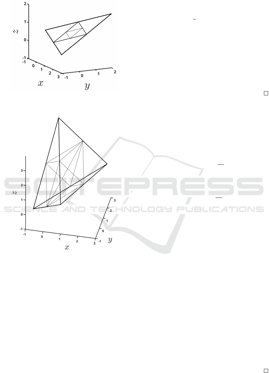
Figure 3: A triangle (2-simplex) in 3 dimensions subdivided

into 2

= 4 triangles, of which one is further subdivided into

= 4 triangles.

Figure 4: A tetrahedron (3-simplex) in 3 dimensions subdi-

vided into 2

= 8 tetrahedra.

Note that Test for Positivity 6 might end up in

an inﬁnite loop if g is non-negative but zero at some

points in S. However, we will show that it always

gives a deﬁnite answer for CPQ Lyapunov function

candidates in the rest of this section.

Deﬁne the diameter of a simplex S =

co{x

,. . . ,x

} ⊂ R

diam(S) := max

i, j=0,1,...,m

∥x

− x

∥

Lemma 7. Let S := co{x

,. . . ,x

} ⊂ R

be an

m-simplex and S

, k = 1,2, 3, . ..,2

, be the simplices

S is subdivided into using the algorithm from Section

4. Let S(x) = Fx + x

be the mapping (18) that maps

the vertices of S

⊂ R

to the vertices of S. Then

diam(S

) ≤

max

y,z∈{0,2}

∥F(y − z)∥

(19)

for k = 1,2,3,..., 2

Proof. First note that all vertices of all simplices in

, σ ∈ S

, are vectors in the set {0,a}

. Since

S(y) − S(z) = F(y − z) and S = F(S

) is subdi-

vided into simplices of the form F(1

+ S

), σ ∈ S

which are congruent to the simplices in F(S

), σ ∈

, which in turn are congruent to the simplices in

F(S

), σ ∈ S

, scaled down by a factor 1/2, the es-

timate (19) follows.

This lemma has an obvious corollary; just set A :=

max

y,z∈{0,2}

∥F(y − z)∥

Corollary 8. Let S := co{x

,. . . ,x

} ⊂ R

be an

m-simplex. Then there is a constant A > 0 such that

if S is K times iteratively subdivided into simplices

using the algorithm from Section 4, i.e. subdivided,

then the simplices in the subdivision are subdivided,

etc., then

diam(S

) ≤

for every simplex S

, k = 1,2,3,.. . , 2

, in the Kth

iteration. In particular

|[x − y]

| ≤

for every two vectors in S

and r = 1,2, . ..,n.

Another obvious corollary, and useful for our pur-

poses, is the following.

Corollary 9. If g in Lemma 3 fulﬁlls g(x) > 0 for all

x ∈ S and if the E

s from Lemma 3 are scaled down

in the obvious way in the iterations (jump from Step

2 to Step 1) in Test for Positivity 6, then the test will

deliver the results g(x) ≥ 0 for all x ∈ S in a ﬁnite

number of steps.

Proof. This is indeed obvious from what we have

shown. The only problem in the formulation is the

inequality (8), as one could successively chose more

and more conservative bounds E

in the iterations.

However, since the upper bounds B

cannot become

larger when we go to smaller simplices, and the terms

|[x

− x

]

| can be scaled down by a factor of 1/2

in each iteration, this is unnecessary and makes no

sense. Hence, we can let the E

converge to zero

uniformly over the iterations and then, at the latest

in the iteration when all E

s are less than or equal

to min

x∈S

g(x) > 0, Test for Positivity 4 in Step 1

of Test for Positivity 6 delivers that g(x) ≥ 0 for all

x ∈ S.

ICINCO 2025 - 22nd International Conference on Informatics in Control, Automation and Robotics

442

Not only will Test for Positivity 6 deliver an afﬁr-

mative answer if g(x) > 0 for all x ∈ S, but if there

is a y ∈ S such that g(y) < 0, then the test will also

deliver the results that g(x) ≥ 0 for all x ∈ S is false,

in a ﬁnite number of steps.

Lemma 10. If for g in Lemma 3 there is a y ∈ S such

that g(y) < 0, then Test for Positivity 6 will deliver a

point y

∗

∈ S such that g(y

∗

) < 0 in a ﬁnite number of

steps.

Proof. Since g is continuous there is an open neigh-

borhood U ⊂ S of y such that g(x) < 0 for all x ∈ U,

and since S from (18) is continuous the set S

−1

(U) is

open in S

⊂ R

and there is an open ball B ⊂ S

where g ◦ S is negative. Now consider that the ver-

tices of S

are the set {0,2}

∩ S

, the set of all

vertices of all the simplices in the ﬁrst subdivision of

is {0,1,2}

∩ S

, the set of all vertices of all

the simplices in the second iterative subdivision of

is {0,1/2, 1, 3/2, 2}

∩ S

, etc. Now, for a large

enough K ∈ N, there must exist an

∗

∈



,. . . ,

2 ·2

− 1



∩ B

and with y

∗

= S(x

∗

) we have 0 > (g ◦ S)(x

∗

) = g(y

∗

Assume V is a CPQ Lyapunov function candidate,

i.e. is of the form (1) and fulﬁlls the conditions (3). In

Theorem 1 we showed that if V (x) ≥ 0 for all x ̸= 0

then V (x) > 0 for all x ̸= 0

0. Hence, for every ν ∈ I,

either V (x) > 0 for all x ∈ C

\ {0

0} or there exists a

y ∈ C

such that V (y) < 0. Combining Corollary 9

and Lemma 10 with these results delivers:

Theorem 11. For a CPQ Lyapunov function candi-

date V of the form (1) that fulﬁlls the conditions (3),

the Test for Positivity 6 is non-conservative when ver-

ifying the conditions (2) for a CPQ Lyapunov func-

tions. That is, the test will give an afﬁrmative answer

in a ﬁnite number of steps, whether (2) holds true or

not.

6 CONCLUSIONS

For switched, cone-wise linear systems, either arbi-

trary switched or with state-dependent switching, we

presented an algorithm to verify the positive deﬁnite

conditions for CPQ Lyapunov function candidates pa-

rameterized using LMIs or LP. Further, we proved in

Theorem 11 that the algorithm is non-conservative,

in comparison to earlier approaches that do introduce

some conservatism. In a subsequent publication we

will describe an efﬁcient implementation of our algo-

rithm for n-dimensional system and demonstrate its

applicability. Further, we will compare its numeri-

cal efﬁciency with the LMI approaches presented in

(Kruszewski et al., 2009; Sala and Arino, 2007; Gon-

zaleza et al., 2017), which are sufﬁcient and asymp-

totically necessary.

ACKNOWLEDGEMENT

We thank the anonymous reviewers for useful sugges-

tions and references.

REFERENCES

Andersen, S., August, E., Hafstein, S., and Piccini, J.

(2023a). Lyapunov function computation for linear

switched systems: Comparison of SDP and LP ap-

proaches. In Proceedings of the 13th International

Conference on Simulation and Modeling Methodolo-

gies, Technologies and Applications, volume 1, pages

61–70.

Andersen, S., Giesl, P., and Hafstein, S. (2023b). Com-

mon Lyapunov functions for switched linear systems:

Linear programming-based approach. IEEE Control

Systems Letters, 7:901–906.

Andersen, S., Hafstein, S., Roman, J., and van den Eijn-

den, S. (2024). Efﬁcient implementation of piece-

wise quadratic Lyapunov function computations for

switched linear systems. In Proceedings of the 21tst

International Conference on Informatics in Control,

Automation and Robotics (ICINCO),, volume 1, pages

277–284.

Camlibel, M. and Pang, S.-J.and Shen, J. (2006).

Conewiselinear systems: Non-zenoness and observ-

ability. SIAM Journal on Control and Optimization,

45(5):1769–1800.

Deenen, D., Sharif, B., van den Eijnden, S., Nijmeijer, H.,

Heemels, M., and Heertjes, M. (2021). Projection-

based integrators for improved motion control: For-

malization, well-posedness and stability of hybrid

integrator-gain systems. Automatica, 133:109830.

Filippov, A. (1988). Differential Equations with Discon-

tinuous Right-hand Side. Kluwer. Translated from

Russian, original book from 1985.

Giesl, P., Hafstein, S., and Pokkakkillath, S. (2025). Piece-

wise quadratic Lyapunov functions for stochastic dif-

ferential equations by linear programm. Discrete Con-

tin. Dyn. Syst. Ser. B, 30(6):2027–2050.

Gonzaleza, T., Sala, A., Bernal, M., and Robles, R.

(2017). Piecewise-Takagi–Sugeno asymptotically ex-

actestimation of the domain of attractionof nonlinear

systems. J. Frank. Inst., 354:1514–1541.

Hafstein, S. (2019). Simulation and Modeling Method-

ologies, Technologies and Applications, volume 873

of Advances in Intelligent Systems and Computing,

Verifying Positivity of Piecewise Quadratic Lyapunov Functions

443

chapter Fast Algorithms for Computing Continuous

Piecewise Afﬁne Lyapunov Functions, pages 274–

299. Springer.

Ikramov, K. and Saveleva, N. (2000). Conditionally deﬁnite

matrices. J. Math. Sci., 98(1):1–50.

Johansson, M. (1999). Piecewise Linear Control Systems.

PhD thesis: Lund University, Sweden.

Johansson, M. and Rantzer, A. (1998). Computation of

piecewise quadratic Lyapunov functions for hybrid

systems. IEEE Trans. Automat. Control, 43(4):555–

559.

Kruszewski, A., Sala, A., Guerra, T., and Arino, C. (2009).

A triangulation approach to asymptotically exact con-

ditions for fuzzy summation. IEEE Trans. Fuzzy Syst.,

17(5):985–994.

Marinósson, S. (2002). Stability Analysis of Nonlin-

ear Systems with Linear Programming: A Lyapunov

Functions Based Approach. PhD thesis: Gerhard-

Mercator-University Duisburg, Duisburg, Germany.

Palacios Roman, J., Hafstein, S., Giesl, P., van den Eijnden,

S., Andersen, S., and Heemels, M. (2024). Construct-

ing continuous piecewise quadratic Lyapunov func-

tions with linear programming. [Submitted].

Sala, A. and Arino, C. (2007). Asymptotically necessary

and sufﬁcient conditions for stability andperformance

in fuzzy control: Applications of Polya’s theorem.

Fuzzy Sets Syst., 158:2671–2686.

Scherer, C. (2006). LMI relaxations in robust control. Eur.

J. Control, 12:3–29.

van den Eijnden, S., Heemels, M., Nijmeijer, H., and Heert-

jes, M. (2022). Stability and performance analysis of

hybrid integrator–gain systems: A linear matrix in-

equality approach. Nonlinear Analysis: Hybrid Sys-

tems, 45:101192.

van den Eijnden, S., Heertjes, M., Heemels, M., and Ni-

jmeijer, H. (2020). Hybrid integrator-gain systems:

A remedy for overshoot limitations in linear control?

IEEE Control Systems Letters, 4(4):1042 – 1047.

Walter, W. (1998). Ordinary Differential Equation.

Springer.

ICINCO 2025 - 22nd International Conference on Informatics in Control, Automation and Robotics

444