Approximating MPC Solutions Using Deep Neural Networks:

Towards Application in Mechatronic Systems

Edward Kikken, Jeroen Willems, Branimir Mrak and Bruno Depraetere

Flanders Make, Lommel, Belgium

Keywords:

Optimal Control, Motion Control, Trajectory Planning, Artiﬁcial Neural Networks, Mechatronics.

Abstract:

Model Predictive Control is an advanced control technique that can yield high performance, but it is often

challenging to implement. Especially for systems with dynamics that are complex to model, have strong non-

linearities, and/or have small time constants, it is often not possible to complete the needed online optimizations

fast and reliable enough. In this work we look at approximating the MPC solutions using black-box models

i.e. deep neural networks, so that the computational load at runtime is strongly reduced. We use a supervised

learning approach to train these models to yield outputs similar to those of an example dataset of ofﬂine

pre-computed MPC solutions. We illustrate this approach on three realistic (active-suspension system, parallel

robot, and a truck-trailer), illustrating the typical workﬂow and how the approach has to be set up to address the

varying challenges. We show that the approximate MPC solutions yield a high level of performance, reaching

nearly the level of the original MPC, yet at a strongly reduced computational load.

1 INTRODUCTION

There is an increasing need for advanced control,

due to stricter requirements for accuracy, productivity

and/or energy efﬁciency, as well as systems becom-

ing more complex and being used in more variable

conditions. One option to achieve this is Model Pre-

dictive Control (MPC). This is a powerful technique

that, during operation, at every time step, chooses the

best control action by solving a numerical optimiza-

tion problem, using a model for the system dynamics

to evaluate the impact of the different control choices

on the constraints and the cost function (Rawlings,

2000). One of the key drawbacks of MPC is the com-

putational burden associated with the aforementioned

optimization. As a result, MPC becomes too slow

and/or too difﬁcult to run on industrial controllers, es-

pecially for (i) systems with small time constants, (ii)

systems with many states, and/or (iii) systems with

highly non-linear dynamics (for which MPC is often

denoted NMPC).

This can be resolved in two different manners.

Firstly, the MPC can be improved, by e.g., simplifying

the models, or by improving the used optimization

routines so they converge more quickly and more reli-

ably (Vanroye et al., 2023). Secondly, and what this

paper will focus on, is to not solve the MPC itself dur-

ing machine operation, but to instead pre-calculate and

approximate its solution, so that during machine op-

eration the calculation of the control does not involve

the solving of an online optimization problem.

Already several works have looked at such ap-

proaches for pre-calculating MPC solutions. Histori-

cally, explicit MPC was developed in (Bemporad et al.,

2000). In this and later works, it was shown that for

an MPC applied to a system with afﬁne dynamics

and constraints, as well as a quadratic cost, the con-

trol output is a piecewise afﬁne function of the states.

The MPC solution is then essentially equal to a set

of linear controllers, depending on the current system

state. And crucially, these can all be pre-calculated

and stored in a big look up table. The main draw-

backs of this approach are (i) the exponential scaling

of the number of needed regions as a function of the

problem size, and (ii) the lack of support for general

non-linear dynamics. Due to the ﬁrst, approximations

of non-linear dynamics cause explicit MPC to quickly

become non-tractable.

In an attempt to address these issues, several works

have looked at approximating the MPC solutions, in-

stead of trying to exactly describe them. Approxi-

mations have been built using for example polynomi-

als (Kvasnica et al., 2011) or multi-scale basis func-

tions (Summers et al., 2011). Recently, neural net-

works have also been considered. For example, com-

bined with a learning scheme to adapt weights and

Kikken, E., Willems, J., Mrak, B. and Depraetere, B.

Approximating MPC Solutions Using Deep Neural Networks: Towards Application in Mechatronic Systems.

DOI: 10.5220/0013712900003982

Paper published under CC license (CC BY-NC-ND 4.0)

In Proceedings of the 22nd International Conference on Informatics in Control, Automation and Robotics (ICINCO 2025) - Volume 1, pages 71-81

ISBN: 978-989-758-770-2; ISSN: 2184-2809

biases to capture optimal control outputs (Parisini

and Zoppoli, 1995), and MPC solutions (Winqvist

et al., 2021; Chen et al., 2018). Some more recent

works have switched to using supervised learning, to

directly learn from examples generated using an MPC

or NMPC controller ofﬂine (Hertneck et al., 2018; Nu-

bert et al., 2020; Lucia et al., 2021). In recent works

such an approach has been applied to non-linear sys-

tems as well as linear ones (Hertneck et al., 2018; Lu-

cia and Karg, 2018). Several works have also looked at

describing or bounding the accuracy or suboptimality

of the solutions (Hertneck et al., 2018), trained sec-

ondary networks (Zhang et al., 2019) to indicate when

suboptimality or even infeasibility becomes an issue,

or proposed architectures relying on cloud-based su-

pervision (Adamek and Lucia, 2023). Recent work

has also looked at ﬁne-tuning such methods after de-

ployment (Hose et al., 2024).

Such Approximate MPC or A-MPC has been

applied to various applications, including building

HVAC (Karg and Lucia, 2018), a polymerization (Lu-

cia and Karg, 2018) and a stirred tank reactor (Hert-

neck et al., 2018), step down (Maddalena et al., 2020)

and resonant power convertors (Lucia et al., 2021),

robots (Nubert et al., 2020), and battery charging

(Pozzi et al., 2022). Our contribution is to apply it

to several more and diverse examples: one straightfor-

ward, one with a ﬁnite task and an economical cost,

and one on path planning with two families of differ-

ing solutions. These later two introduce challenges

not tackled in the existing examples, and we propose

several A-MPC changes to handle those. To tackle

the ﬁnite tasks we provide the A-MPC with extra in-

formation on the remaining task, allowing the net-

work to adapt during the execution. To tackle the

path planning we treat the A-MPC as a mixed integer

control problem, and add a classiﬁer for the integer

values. This differs from existing approaches like us-

ing deeper networks (Karg and Lucia, 2018), or using

stochastic (Bernoulli) layers to handle integer vari-

ables (Okamoto et al., 2024). Furthermore we will

look into the trade-off between the number of MPC

training examples and the resulting A-MPC perfor-

mance, since in practice generating data for training

these A-MPC takes signiﬁcant time. Detailed statisti-

cal analysis of robustness for these applications will

however be left to future work.

2 PRELIMINARIES

In this section, we ﬁrst introduce the mathematical no-

tation considered in this paper, and then give a generic

MPC formulation, on which we will build further.

2.1 Notation

We denote

as the set of real vectors of dimension

, and

m×n

as the set of real matrices of dimension

m × n

. A control sequence [

· · · u

]

∈ R

is denoted by the bold vector u with

N ∈ N

discrete

samples. A speciﬁc sample is given by integer

(

)

with k ∈ N.

2.2 Generic Model-Predictive Control

(MPC)

Model Predictive Control (MPC) is a generic class

of control methods which utilize a dynamic model to

predict the future response of the system, and choose

the control actions yielding the best predicted response

(given a cost function and constraints). To do so, at

each control interval in a given ﬁnite-time horizon (of

samples), MPC optimizes current and future con-

trols and state trajectories (Qin and Badgwell, 2003).

Once the optimal controls are found, the ﬁrst values

are applied at the current time-step, the system’s re-

sponse is observed, and the MPC is optimized again

starting from the observed system state. This proce-

dure is repeated at every time step, which allows the

MPC to react in a manner similar to feedback control,

to deviations due to e.g., model-plant mismatch and

disturbances. Using the predictive approach it also

becomes straightforward to exploit preview or predic-

tions of upcoming events like disturbances or external

loads.

As said, the MPC relies on a model. Here, we

consider a discrete-time model:

x(k + 1) = f (x(k), u(k)),

(1)

with the dynamic states x(

)

∈ R

and the control

actions u(

)

∈ R

, with

and

the number of states

and inputs respectively. In the above,

denotes the

state propagation function (e.g., ordinary differential

equation (ODE)). This generic function can be linear

or non-linear, SISO or MIMO, etc.

This model can then be used to set up the MPC

formulation. Here, we use a horizon of

N ∈ N

intervals

(samples), yielding:

minimize

x(·),u(·)

J (x(·), u(·)), (2a)

s. t. (1) ∀ k ∈ [1, N],

(2b)

x ≤ x(k) ≤

x ∀ k ∈ [1, N + 1],

(2c)

u ≤ u(k) ≤

u ∀ k ∈ [1, N],

(2d)

g ≤ g(x(·), u(·), y(·), p) ≤

g. (2e)

ICINCO 2025 - 22nd International Conference on Informatics in Control, Automation and Robotics

with cost function

(·),

(·)

). Matrix x

(·) ∈

×N+1

contains the optimization variables over

the entire horizon for the differential states: x

(·)



, x

, . . . , x

, x

N+1



, and u

∈ R

×N

similarly con-

tains all control actions. In the above, (2a) implements

the cost function, (2c) and (2d) implement lower and

upper bounds on the state and input variables, and

(2e) implements miscellaneous constraints (e.g., initial

condition and path constraints).

As mentioned previously, MPC solves the opti-

mization problem denoted in (2) at every time step.

After solving, the ﬁrst sample of the computed input

sequence u

(·)

is then applied to the system, i.e., u

(1)

and we again solve the optimization problem for the

next time sample.

3 PROPOSED APPROACH

Our proposed approach to approximate MPC solutions

using black-box models, namely deep neural networks

(DNN) consists out of three steps:

Ofﬂine, we formulate the MPC problem (see Sec-

tion 2.2) for the use-case at hand and solve it for a

large combination of states, constraints, possibly

model-variants, etc. The goal is to capture the de-

sired operating region of the system / task. The

result is an input dataset

containing the system

states and additional features like e.g. obstacle

locations or the time left to task completion, and

an output dataset

containing the optimal control

actions as computed by the MPC.

Still ofﬂine, DNN is trained that aims to approxi-

mate the mapping from input dataset

to output

dataset U.

At run-time, DNN is used to calculate the plant

input as a function of the current input features, and

aims to act as a direct replacement to the original

MPC controller.

3.1 MPC Problem Formulation and

Dataset Generation

In order to set-up the MPC for a given application,

we use the template from Section 2.2 and implement

application-speciﬁc costs and constraints. We use

CasADi (Andersson et al., 2019) to set-up the mod-

els and optimization problems, and the solver IPOPT

(Biegler and Zavala, 2009) is used to efﬁciently solve

the problem.

As mentioned previously, the goal is to create two

datasets:

•

Input dataset

X ∈ R

×M

containing

∈ N

fea-

tures, such as states, as well as additional features

like current sample in the task and time to com-

pletion, potentially a preview of upcoming distur-

bances or other external signals relevant to the con-

troller, locations of obstacles, etc.

M ∈ N

denotes

the total number of MPC solutions in the dataset.

•

Output dataset

U ∈ R

×M

containing the optimal

control actions (e.g. torques, forces, trajectories).

∈ N denotes the number of outputs.

The goal is to generate a rich dataset, covering the

states, inputs, etc. of interest. The richer the datasets,

the better the approximate controller will perform in a

variety of unseen conditions, but the higher the compu-

tational effort required to build the dataset and to train

the DNN. To address this, we followed an iterative

approach for building our dataset. We ﬁrst deﬁned a

bounded region of realistic values for states, inputs,

etc. Then, we started with a relatively compact dataset

of MPC solutions i.e.,

and

, sampled from the

complete region of operation and used these to ﬁt a

DNN. Afterwards, we analyzed the performance on

a wide set of test points

val

within the desired re-

gion of operation but which are not included in

If the performance on

val

is not yet sufﬁcient more

points were added thereby increasing the density of

, until the performance is sufﬁcient. This was done

in ad-hoc manner since this paper focuses on the ap-

plications, but more thorough statistical analysis of

performance for training set size has been performed

in e.g. (Hertneck et al., 2018). We also used random

samples of states or trajectories through the operation

space. Through optimal design of experiments (DoE),

a more targeted choice could be made regarding this

trade-off, like in (Gupta et al., 2023; Chen and Peng,

2017).

3.2 Training Deep Neural Networks

A DNN is trained to ﬁt the mapping from input dataset

to output dataset

. Various design choices can

be made, e.g., the type of network (DNN, possibly in

tandem with additional networks as classiﬁers), the

corresponding architecture and its hyperparameters.

Typically, the appropriate choice of the architecture

follows from the complexity of the considered use-

case.

In the most basic format, we consider a feedfor-

ward neural network, because of its general purpose na-

ture. The neural network architecture includes an input

layer with

input features,

layers

fully-connected

hidden layers each containing

hidden

neurons, and

an output layer with

output features representing

the control actions. All layers are fully connected. In

Approximating MPC Solutions Using Deep Neural Networks: Towards Application in Mechatronic Systems

between the layers, we use activation functions, e.g.,

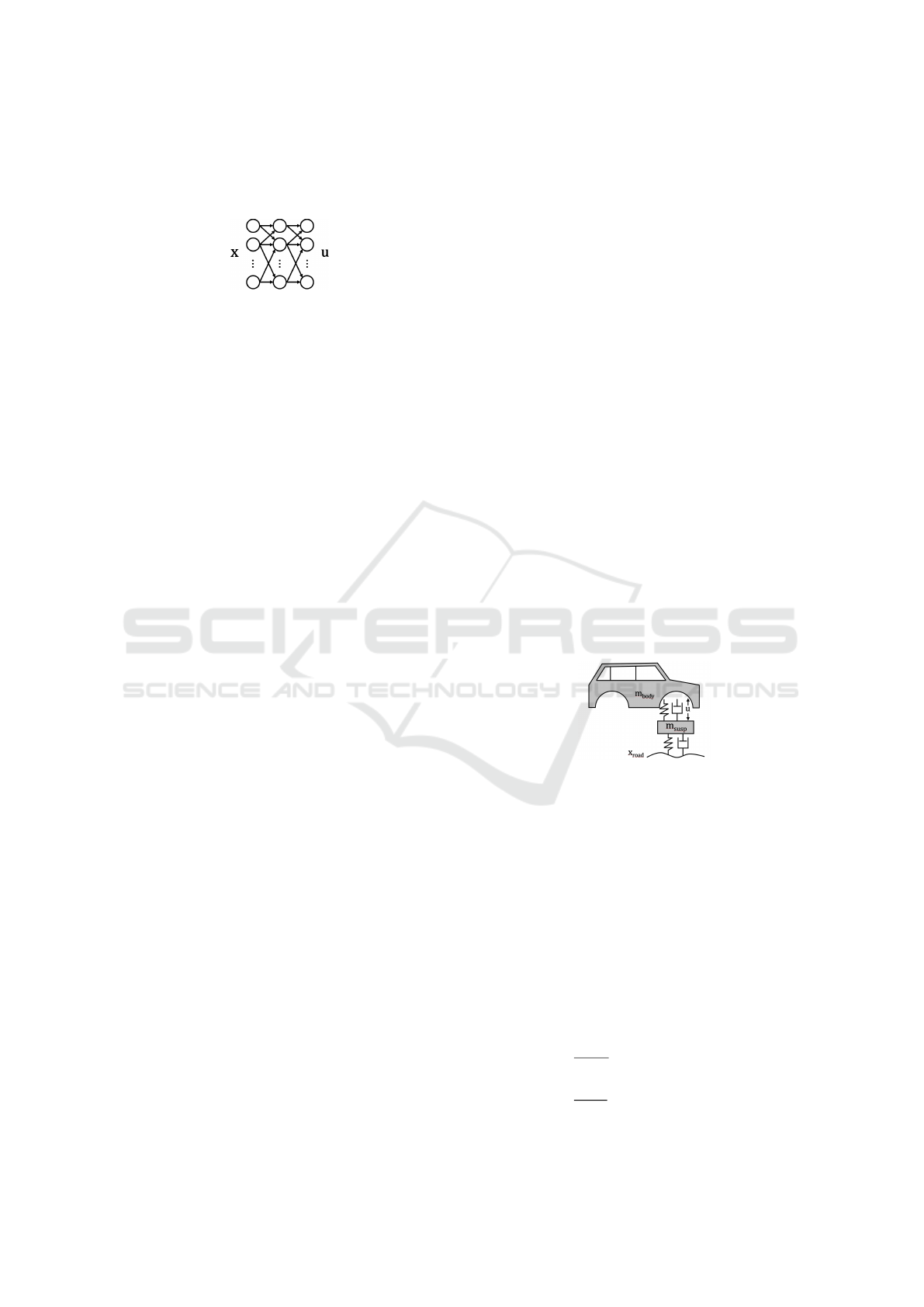
ReLU or Tanh. A simple example of such a neural

network is shown in Figure 1.

Figure 1: A simple multi-layer feedforward neural network

mapping inputs to outputs.

We implement DNN models using Torch (Paszke

et al., 2019) and use the Adam optimizer (Kingma and

Ba, 2014) to optimize the weights and biases. The cost

function used to train the DNN is the mean squared

error between the output features in

and the model’s

predictions. After scaling the input and output datasets,

the training is ran for a number of epochs until the

ﬁtting error is sufﬁciently low.

3.3 Deployment

After the DNN has been trained using the approach

in Sections 3.1 and 3.2, it can be deployed on the

machine controller. There it receives online measure-

ments and computes its approximate MPC control ac-

tions, thereby replacing the original MPC.

4 VALIDATION

In this section, we validate the proposed algorithm on

a range of use-cases:

•

An active-suspension system, where the suspen-

sion is controlled to optimize comfort, while sub-

ject to road variations. This is a simple linear case

to start with, with a relatively small timescale, and

a classical quadratic cost of states and control ac-

tions.

•

A parallel SCARA robot, executing energy-

optimal point-to-point motions while avoiding an

obstacle. This is a more complex case, with non-

linear dynamics, a lower time constant, and a ﬁnite

task to be completed.

•

A truck-trailer, which has to make a U-turn in a

tight space. This is an even more challenging case,

due to the non-linear dynamics, and since the (in-

teger) numbers of reversals is not the same for all

possible turns.

The performance difference between the two ap-

proaches can be addressed on multiple fronts:

•

Performance in terms of cost and constraints. The

results can be compared to the original MPC ones,

initially on training data to study the impact of

ﬁtting errors, and then on validation data.

•

Computational efﬁciency. The goal of the ap-

proach is to reduce the computational effort re-

quired during run-time. Nevertheless, the proposed

method requires an increased pre-calculation cost

for building the training set and training the net-

work. Here we use the needed calculation time

for both, but ideally this should be done based on

FLOPS.

For each of the examples, we assume all states are

measurable without noise and / or disturbances. In

practice, it can be needed to add estimators to obtain

these, like for most MPC implementations.

4.1 Active-Suspension System

In this section, we consider the active suspension use-

case. The suspension system can be controlled to

manage the vertical movement of the car. Unlike pas-

sive suspension systems, which rely on ﬁxed springs

and dampers, active suspension systems are able to

adjust in real-time to the road conditions and driving

dynamics, thereby improving passenger comfort. The

considered system is modeled as a quarter car, shown

schematically in Figure 2. It consists of a car body and

a suspension, driving on a given road.

Figure 2: The considered quarter car with active suspension.

The system has 5 states:

x =



body

susp

road



∈ R

and 2 inputs:

u =



susp

road



∈ R

where

and

denote displacement, speed and input

force respectively. The linear dynamics are given in

ODE format as:

˙x

road

= v

road

˙x

body

= v

body

˙x

susp

= v

susp

˙v

body

(−F

susp

+ u

susp

)),

˙v

susp

(+F

susp

− u

susp

+ F

road

)),

(3)

ICINCO 2025 - 22nd International Conference on Informatics in Control, Automation and Robotics

where:

susp

= d

susp

body

− v

susp

) + k

susp

body

− x

susp

and:

road

= d

tire

road

− v

susp

) + k

tire

road

− x

susp

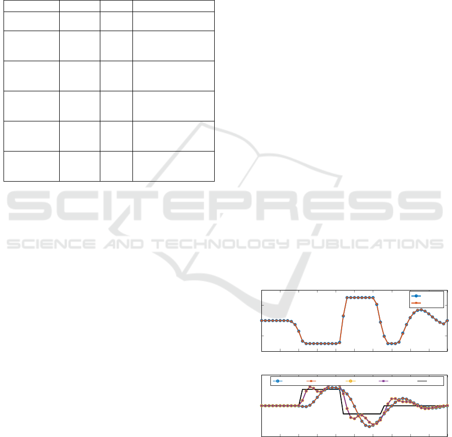
The model parameters are shown in Table 1.

Table 1: Model parameters for the active suspension.

Parameter Value Unit Description

body

625 kg

Body mass (25%)

susp

320 kg

Mass of

suspension

susp

0 Ns/m

Damping constant

of suspension

tire

3755 Ns/m

Damping constant

of wheel and tire

susp

80000 N/m

Spring constant

of suspension

tire

125000 N/m

Spring constant

of wheel and tire

The control goal of the MPC is to minimize the

displacement of the car body,

body

, by controlling

susp

. Therefore, the cost function (Eq. 2a) is set to:

J = w

i=N

∑

i=1

body

(i)

+ w

i=N

∑

i=1

susp

(i)

Scalar weights

∈ R

and

∈ R

trade off the two

cost functions: minimization of displacement and in-

put regularization respectively. The constrains are

given by:

•

Initial condition: x

= x

current

, i.e., the initial state

of the optimization problem is set to the current

state of the system.

• Input constraint: −3000 ≤ u

susp

≤ 3000.

We consider a sampling time of 0.04 s and an MPC

horizon of 0.2 seconds (

= 5 samples). A forward

Euler integrator is used to integrate the dynamics. The

MPC receives preview of the road proﬁle (

road

and

road

) 5 samples ahead.

After setting up the MPC, it is run for a grid of con-

ditions to construct input dataset

to output dataset

U, which contain the following features:

•

The input features are selected as the 5 states at the

current sample, and 5 samples ahead (preview) of

road

•

A single output feature is considered: the next

sample of u

susp

In total, 1000 MPC solutions are generated by varying

the input features as follows:

•

The ﬁrst 4 states are excited at



−0.3 0 0.3



and the last state at



−0.1 0 0.1



•

The road proﬁle,

road

, is excited at



−3 0 3



for each of the samples.

Note that a full factorial sampling grid is considered,

but that the coverage is relatively sparse. Due to the

linear dynamics of the system, the model trained next

performs well at intermediate points, removing the

need for additional intermediate samples in the training

data.

The considered neural network is designed as a

feed-forward neural network consisting of 2 fully

connected hidden layers with 20 neurons each, with

ReLU activation functions. After training, a root-mean-

squared error of 18 N is achieved on the training data

(0.85%) Next, the result is tested / deployed for a given

road proﬁle with a length of 50 samples (10 times the

MPC horizon), and benchmarked with the MPC so-

lutions. In Figure 3, the results are shown. It can

be seen that the solution of the proposed approach

closely matches that of the original MPC, also if the

input constraints are active. In terms of the cost, the

original MPC has a cost of 0.127, while the MPC-

approximation has a 0.5 percent higher cost. Regard-

ing evaluation time: evaluating the original MPC takes

33 ms per iteration, while the proposed A-MPC ap-

proximation only requires 0.5 ms per iteration, which

is limited by our non real-time operating system and

is expected to be signiﬁcantly faster on a typical em-

bedded controller.

0 0.2 0.4 0.6 0.8 1 1.2 1.4 1.6 1.8 2

−4,000

−2,000

2,000

4,000

Time [s]

Force [N]

MPC

A-MPC

0 0.2 0.4 0.6 0.8 1 1.2 1.4 1.6 1.8 2

−0.15

0.15

Time [s]

Displacement [m]

MPC (b) A-MPC (b) MPC (s) A-MPC (s) Road

Figure 3: Validation on a given road proﬁle. (b) denotes the

body, (s) denotes the suspension.

Approximating MPC Solutions Using Deep Neural Networks: Towards Application in Mechatronic Systems

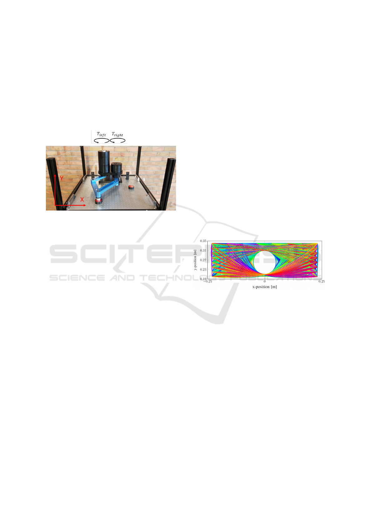
4.2 Parallel SCARA

In this section, we consider a parallel SCARA robot,

shown in Figure 4. Such a system is often used for

pick-and-place or assembly operations, where high

speed and accuracy are required. The considered sys-

tem is driven by two motors, and controls the location

of an end-effector. The system has non-linear dynam-

ics and is MIMO, making it challenging to control.

Figure 4: The considered SCARA setup.

The system is driven by two motors (left and right),

yielding motor torques u =



le f t

right



∈ R

, and

controls the position of an end-effector, yielding states

x =



˙x

˙y



∈ R

. In this paper, we con-

sider a simulation study, based on a model designed

using ROBOTRAN (Docquier et al., 2013). For the

sake of brevity, we refer to (Singh et al., 2024) for the

detailed model equations.

For this case, the control goal of the MPC is to con-

duct a point-to-point motion, from a given initial end-

effector state (x

init



init

0 y

init



) to a ﬁnal

end effector state (x

end



end

0 y

end



), while

minimizing the required input torque. Therefore, the

cost function (Eq. 2a) is set to minimize the torques:

J =

i=N

∑

i=1

le f t

(i)

i=N

∑

i=1

right

(i)

. (4)

The constrains are given by:

•

Initial condition: x

= x

current

, i.e., the initial state

of the optimization problem is set to the current

state of the system. For the ﬁrst sample of the task,

= x

init

•

Obstacle avoidance: the end-effector has to stay

outside of a given constraint surface: a circle with

a radius of 0.05 m, illustrated later.

There is also the constraint to ensure the robot reaches

the desired target x

end

at the end of the task length,

which is 0.25 s. To do so, we re-solve the MPC every

sample with a sampling time of 0.0025 s, and as the

task is executed, each time, the length of the MPC

horizon

is decreased by 1, going from 100 initially

down to 1 as the task is completed.

We consider the following features for input dataset

X to output dataset U:

•

The input features are selected as the current states

current

, the desired ﬁnal positions of the end-

effector,

end

and

end

, and ﬁnally also the (integer)

number of samples until the end of the total task

horizon. This last feature provides a notion of how

many samples are left until the end of the task.

•

Two output features are considered: the motors

torques T

le f t

and T

right

The datasets

and

are constructed by varying

the initial and ﬁnal condition (end-effector positions)

of the point-to-point motion. We vary the initial and

ﬁnal x-position between -0.23 and 0.23 m in 8 steps.

Similarly, we vary the y-position between 0.20 and

0.34 m in 8 steps, yielding a number of 4096 conﬁg-

urations. Each of the conﬁgurations has a task length

of 100 samples, so in total we have 409600 MPC so-

lutions. All trajectories, including the obstacle, are

visualized in Figure 5 where it can be seen that the

training data covers the region of interest densely.

Figure 5: The generated trajectories, including the obstacle.

Again, we consider a feed-forward neural network,

but in this case it consists of 2 fully connected hid-

den layers with 150 neurons, with ReLU activation

functions. After training, a root-mean-squared error of

0.14 Nm is achieved on the training dataset.

In order to test the proposed approach we consider

two cases. First, we will consider an initial and ﬁnal

point within the training data. Second, we consider an

intermediate point, to investigate how well the algo-

rithm extrapolates to unseen conditions.

The ﬁrst case considers

init

= 0

23,

init

= 0

and

end

−

23,

end

= 0

2, which are direct mem-

bers of the training data. With respect to the cost

function, the original MPC has an RMS torque of 0.82

Nm and the A-MPC an RMS torque of 0.83 Nm.

The second case considers

init

−

13,

init

33 and

end

= 0

13,

end

= 0

23. In this case, the

initial and ﬁnal conditions are placed relatively far way

from the grid points in the training dataset, aiming to

investigate how well the proposed algorithm general-

ICINCO 2025 - 22nd International Conference on Informatics in Control, Automation and Robotics

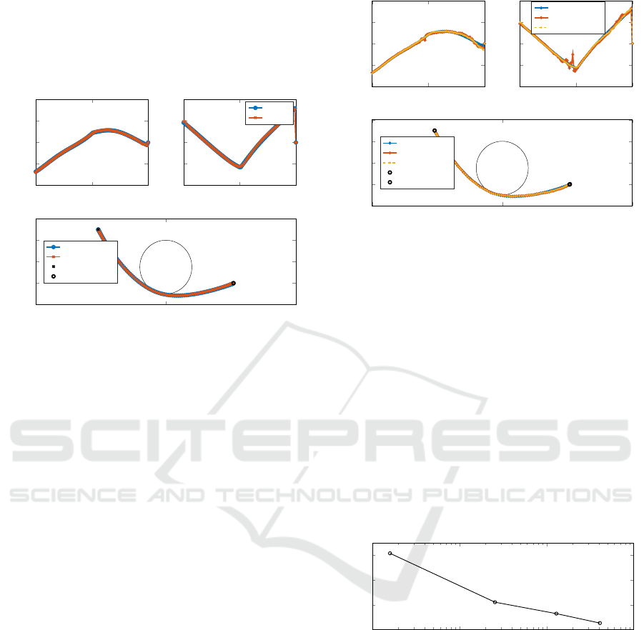
izes to unseen data. In Figure 6, the results are shown.

In the ﬁgure, it can be seen that the solutions are still

very similar. With respect to the cost function, the

original MPC has an RMS torque of 0.660 Nm and the

A-MPC an RMS torque of 0.662 Nm.

0.125 0.25

−10

−5

Time [s]

Torque (left) [Nm]

0.125 0.25

−10

−5

Time [s]

Torque (right) [Nm]

MPC

A-MPC

−0.25

0.25

0.19

0.23

0.27

0.31

0.35

x-position [m]

y-position [m]

MPC

A-MPC

Initial condition

Final condition

Figure 6: Result for conditions outside the training set.

Next, we study the effect of measurement noise on

the performance. To do so, a white noise disturbance

is added to the states (magnitude of 0.5 mm (position)

and 1 mm/s (velocity) respectively). For each of the

controllers, the same noise proﬁle is applied. The

results are shown in Figure 7. The following observa-

tions are made:

•

When noise is added, both the MPC as well as the

A-MPC deviate from the original solution.

•

The obtained input / displacement proﬁles are rel-

atively similar, but the input signal of the MPC

has more oscillations (especially when it nears the

circular constraint). The A-MPC does not display

this effect, since these effects were not accounted

for in the training data.

•

The computed costs for both solutions are the same,

0.665 Nm. However, both solutions do slightly vio-

late the constraints. This will be further dealt with

in future work: by designing an MPC robust to

noise, and by training an A-MPC on the resulting

solutions.

Regarding evaluation time: evaluating the original

MPC takes 40 ms per iteration (on average), while the

MPC approximation only requires 0.5 ms per iteration

(as before limited by our non real-time system). Hence,

the original MPC is on average 16 times slower com-

pared to the sampling time of the system (and thereby

does not meet the real-time requirements), compared

to the proposed approach which is 5 times faster. Note

however that it took approximately 4 hours to generate

the dataset and train the model used for the A-MPC.

0.125 0.25

−10

−5

Time [s]

Torque (left) [Nm]

0.125 0.25

−10

−5

Time [s]

Torque (right) [Nm]

MPC (no noise)

MPC (noise)

A-MPC (noise)

−0.25

0.25

0.19

0.23

0.27

0.31

0.35

x-position [m]

y-position [m]

MPC (no noise)

MPC (noise)

A-MPC (noise)

Initial condition

Final condition

Figure 7: Result for conditions outside the training set, in-

cluding noise.

To arrive at the presented A-MPC performance, we

applied the iterative training data generation approach

from Section 3.1. We varied the initial and ﬁnal

and

positions in either 2, 4, 6 or 8 steps, yielding

increasingly rich training data sets of 16, 256, 1024

and 4096 trajectories, respectively. After each data set

generation we analyzed the root-mean-squared error

of the torques predicted by the A-MPC obtained on

those versus those of the original MPC, on a different

validation dataset, and increased the number of steps

further if accuracy was not yet sufﬁcient. The result

is shown in Figure 8. In the ﬁgure, we can see that

denser input space sampling (and more trajectories in

the training dataset), yields better performance on the

validation set, as is to be expected.

Number of trajectories in training dataset [-]

RMSE (validation) [Nm]

Figure 8: Trade-off between the number of trajectories in the

dataset and the ﬁtting performance on a validation dataset.

4.3 Truck-Trailer

The last case considered in this paper is a truck-trailer,

which has to make a U-turn. Depending on the avail-

able space, it can sometimes be needed to make a

number of speed reversals, but not always. An exam-

ple without reversal is shown in Figure 9, and one with

one speed reversal in Figure 10. For the latter, the

truck moves from a given initial condition with the

truck oriented to the top of the page, to a ﬁnal con-

dition with it oriented down, while subject to space

Approximating MPC Solutions Using Deep Neural Networks: Towards Application in Mechatronic Systems

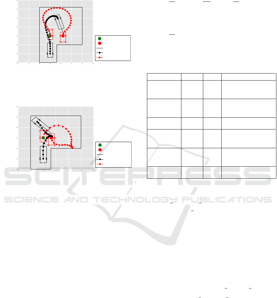
constraints.

−15

−10

−5

−15

−10

−5

x-position [m]

y-position [m]

Initial condition

Final condition

Constraints

Trailer (MPC)

Truck (MPC)

Figure 9: Example of paths for truck and trailer when per-

forming a U-turn without a speed reversal.

−10 −5 0 5 10 15 20

−15

−10

−5

x-position [m]

y-position [m]

Initial condition

Final condition

Constraints

Trailer (MPC)

Truck (MPC)

Figure 10: Example truck-trailer paths with one speed rever-

sal.

In contrast to the previous use-cases discussed in

this paper, we do not consider an MPC which is solved

at each time step in the horizon. Instead, we construct

a model that is able to predict the ideal trajectory (cov-

ering the entire horizon) at once. We do this since

in reality we would then let an external path-tracking

controller track the path, not an MPC, which is left out

of scope for this paper.

The system has 4 states:

x =





∈ R

and 2 inputs:

u =





∈ R

where

and

denote displacements in their respective

direction,

the velocity,

denotes the heading and

the steering angle input. Subscript (

)

denotes the

truck, and subscript (·)

the trailer.

The non-linear dynamics are given in ODE format

as:

sin(β

) −

cos(β

)

tan(δ

˙x

= v

cos(θ

˙y

= v

sin(θ

tan(δ

(5)

where

− θ

. The model parameters are shown

in Table 2.

Table 2: Model parameters for the truck-trailer.

Parameter Value Unit Description

3.5 m

Truck: axle

to axle distance

2 m

Truck: distance

of hitch behind axle

2.5 m

Truck: width

8 m

Trailer: axle to

hitch distance

2 m

Trailer: distance of

axle to rear wall

2.5 m

Trailer: width

For this case, the control goal is to conduct

a point-to-point motion, from a given initial state

init



0 0



) to a ﬁnal state (x

end



(·) x

end

0 −



). Note that the ﬁnal trailer an-

gle θ

is left free.

The considered cost function is to minimize:

J =

i=N

∑

i=1

˙v

so the motion is completed in as smooth a manner as

possible. We consider the following constraints:

•

Initial and ﬁnal condition, as mentioned previ-

ously.

• Steering angle constraint: −

≤ δ

≤

• Relative angle: −

≤ β

≤

• Truck speed: −3 ≤ v

≤ 3.

•

Space constraints:

< y

max

< y

max

> −

< −5.

To solve the optimal control problem, we consider a

sampling time of 1 s and a total task length of

= 30

samples. We solve the entire task at once.

In order to generate the input and output dataset,

we vary

end

∈ R

between 3.25 and 6 m in 12 steps and

max

∈ R

between 8 and 16 m in 33 steps, yielding 396

ICINCO 2025 - 22nd International Conference on Informatics in Control, Automation and Robotics

solutions in total. The resulting truck trajectories (x

and y

) are visualized in Figure 11. All solutions start

from an initial condition of 0 in

- and

-direction. It

can be seen that some solutions have 0 speed reversals,

whereas other solutions have 1. Sometimes, the speed

reversal occurs towards the beginning of the trajectory

(causing the truck to move in negative

-direction) and

sometimes towards the end. The amount of turns is af-

fected by the settings

max

and

end

, further illustrated

later on in this section.

Using this data, we then deﬁne the following fea-

tures that will be used for training the A-MPC:

•

Input features:

end

max

. Note that some of the

initial and ﬁnal states are ﬁxed (eg also

end

varies)

and thus omitted from the dataset, but in general

these would also need to be included as input.

•

Output features: the truck trajectories (with length

N) x

∈ R

, y

∈ R

, v

∈ R

−6 −4 −2 0 2 4 6 8 10 12 14

−10

x-position [m]

y-position [m]

Figure 11: The trajectories of the truck, used for training.

An extra feature that is relevant here is the (inte-

ger) number of speed reversals (0 or 1)

reversals

∈ N

This makes the path planning problem a mixed integer

control problem. Rather than solving this using deeper

networks (Karg and Lucia, 2018), or using stochastic

(Bernoulli) layers (Okamoto et al., 2024), we augment

the neural network with a separate classiﬁer.

To do so, we have chosen a binary classiﬁer to ﬁrst

predict the number of speed reversals, based on input

features:

end

and

max

. Hereby, for simplicity, this is

done using a support-vector machine (SVM), employ-

ing an RBF kernel. In another application use of neural

network classiﬁers could be preferred. The predicted

reversals

by this classiﬁer is used as an input to the next

part of our A-MPC, which is a feed-forward neural

network, consisting of 2 fully connected hidden layers

with 1500 neurons, with ReLU activation functions.

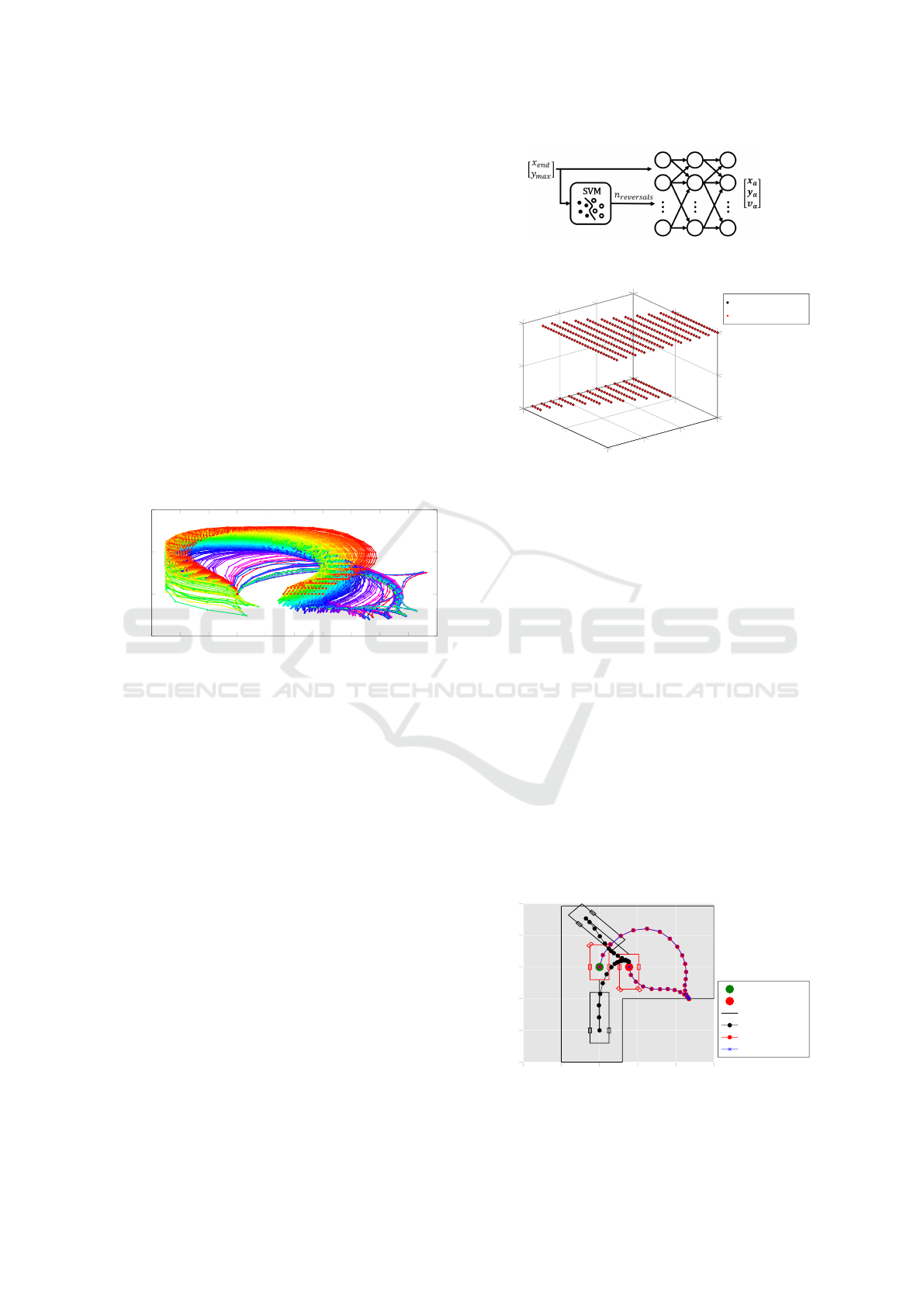
The overall interconnection is shown in Figure 12.

The result of this SVM is shown in Figure 13. For

the training set, it is able to perfectly predict the num-

ber of speed reversals.

Regarding the neural network, it converges to a

root-mean-squared error of 0.017 m for the displace-

Figure 12: The interconnection of the neural network and

SVM.

0.5

end

[m]

max

[m]

Amount of reversals [-]

Reversals (true)

Reversals (pred.)

Figure 13: The amount of speed reversals (true and pre-

dicted), based on the input features.

ment in

- and

-direction (0.25%) and 0.003 m/s for

the truck velocity (0.23%) on the training data.

Next, the approach is ﬁrst validated on a trajectory

for one of the grid points in the training data:

max

16 m,

end

= 6 m. For this case, no speed reversals are

present, not in the optimal solution used for training

and also not in the approximation. With respect to the

trajectories in

- and

-direction, a root-mean-squared

error of 0.01 m is achieved. Next, we consider a tra-

jectory within the same ranges for

max

and

end

, but

not on any of the grid points used for training, with

max

= 9.625 m,

end

= 3.875 m. Now there is one

speed reversal for the approximation, which matches

the outcome of the optimal solution that we ﬁnd when

we calculate it for validation (but this was not used

for training), as shown in Figure 14. In this case, the

root-mean-squared error is small as well: 0.02 m.

Regarding computational effort: solving the MPC

takes on average 3 seconds, whereas inference of the

DNN requires only 3 milliseconds.

−10 −5 0 5 10 15

−15

−10

−5

x-position [m]

y-position [m]

Initial condition

Final condition

Constraints

Trailer (MPC)

Truck (MPC)

Truck (A-MPC)

Figure 14: Validation on conditions outside the training set.

Approximating MPC Solutions Using Deep Neural Networks: Towards Application in Mechatronic Systems

5 CONCLUSION

We have shown application of an approximate MPC

technique on several challenging mechatronics cases.

It relies on supervised learning, to train DNNs to match

MPC examples. This allows to pre-calculate the MPCs,

and thereby reduces the computational load at runtime.

This makes this approach very usable for cases with

complex or non-linear dynamics and/or small time

constants, for which classical MPC would otherwise

typically not be realistic. We have illustrated the versa-

tility of the approach by applying it to several different

examples. We have also shown the workﬂow for how

to tailor the approach for each of those examples, in-

cluding extensions for handling ﬁnite tasks and mixed

integer control problems.

We have worked in a pragmatic manner, but in the

future will work on (i) a thorough stochastic analysis

of training set and optimality or feasibility, allowing

to give stronger validations or even veriﬁcations of

the A-MPC, (ii) more targeted procedures to generate

training data, and (iii) different architectures, wherein

approximations are used alongside classical methods,

for example like in (Chen et al., 2022) where an MPC

is given a feasible initialization using an efﬁcient ap-

proximation.

While we have only reported needed training time

and inference time, it is interesting for future work

to study the ecological impact, tradeing off increased

pre-processing cost with the reduced run-time cost like

done in (Lacoste et al., 2019).

ACKNOWLEDGMENT

This research was supported by: Flanders Make, the

strategic research centre for the manufacturing indus-

try in Belgium, speciﬁcally by its DIRAC SBO and

LearnOPTRA SBO research projects, and the Flemish

Government in the framework of the Flanders AI Re-

search Program (https://www.ﬂandersairesearch.be/en)

that is ﬁnanced by EWI (Economie Wetenschap & In-

novatie).

REFERENCES

Adamek, J. and Lucia, S. (2023). Approximate model predic-

tive control based on neural networks in a cloud-based

environment. In 2023 9th International Conference

on Control, Decision and Information Technologies

(CoDIT), pages 567–572. IEEE.

Andersson, J. A., Gillis, J., Horn, G., Rawlings, J. B., and

Diehl, M. (2019). Casadi: a software framework for

nonlinear optimization and optimal control. Mathemat-

ical Programming Computation, 11(1):1–36.

Bemporad, A., Morari, M., Dua, V., and Pistikopoulos, E.

(2000). The explicit solution of model predictive con-

trol via multiparametric quadratic programming. In

Proceedings of the 2000 American Control Conference.

ACC (IEEE Cat. No.00CH36334), volume 2, pages

872–876 vol.2.

Biegler, L. T. and Zavala, V. M. (2009). Large-scale nonlin-

ear programming using ipopt: An integrating frame-

work for enterprise-wide dynamic optimization. Com-

puters & Chemical Engineering, 33(3):575–582.

Chen, S., Saulnier, K., Atanasov, N., Lee, D. D., Kumar, V.,

Pappas, G. J., and Morari, M. (2018). Approximat-

ing explicit model predictive control using constrained

neural networks. In 2018 Annual American Control

Conference (ACC), pages 1520–1527.

Chen, S. W., Wang, T., Atanasov, N., Kumar, V., and Morari,

M. (2022). Large scale model predictive control with

neural networks and primal active sets. Automatica,

135:109947.

Chen, Y. and Peng, C. (2017). Intelligent adaptive sampling

guided by gaussian process inference. Measurement

Science and Technology, 28(10):105005.

Docquier, N., Poncelet, A., and Fisette, P. (2013). Robotran:

a powerful symbolic gnerator of multibody models.

Mechanical Sciences, 4(1):199–219.

Gupta, S., Paudel, A., Thapa, M., Mulani, S. B., and Wal-

ters, R. W. (2023). Optimal sampling-based neural

networks for uncertainty quantiﬁcation and stochas-

tic optimization. Aerospace Science and Technology,

133:108109.

Hertneck, M., Köhler, J., Trimpe, S., and Allgöwer, F.

(2018). Learning an approximate model predictive

controller with guarantees. IEEE Control Systems Let-

ters, 2(3):543–548.

Hose, H., Brunzema, P., von Rohr, A., Gräfe, A., Schoellig,

A. P., and Trimpe, S. (2024). Fine-tuning of neural net-

work approximate mpc without retraining via bayesian

optimization. In CoRL Workshop on Safe and Robust

Robot Learning for Operation in the Real World.

Karg, B. and Lucia, S. (2018). Deep learning-based embed-

ded mixed-integer model predictive control. In 2018

European Control Conference (ECC), pages 2075–

2080.

Kingma, D. P. and Ba, J. (2014). Adam: A

method for stochastic optimization. arXiv preprint

arXiv:1412.6980.

Kvasnica, M., Löfberg, J., and Fikar, M. (2011). Stabilizing

polynomial approximation of explicit mpc. Automatica,

47(10):2292–2297.

Lacoste, A., Luccioni, A., Schmidt, V., and Dandres, T.

(2019). Quantifying the carbon emissions of machine

learning. arXiv preprint arXiv:1910.09700.

Lucia, S. and Karg, B. (2018). A deep learning-based ap-

proach to robust nonlinear model predictive control.

IFAC-PapersOnLine, 51(20):511–516. 6th IFAC Con-

ference on Nonlinear Model Predictive Control NMPC

2018.

ICINCO 2025 - 22nd International Conference on Informatics in Control, Automation and Robotics

Lucia, S., Navarro, D., Karg, B., Sarnago, H., and Lucía, O.

(2021). Deep learning-based model predictive control

for resonant power converters. IEEE Transactions on

Industrial Informatics, 17(1):409–420.

Maddalena, E., da S. Moraes, C., Waltrich, G., and Jones,

C. (2020). A neural network architecture to learn ex-

plicit mpc controllers from data. IFAC-PapersOnLine,

53(2):11362–11367. 21st IFAC World Congress.

Nubert, J., Köhler, J., Berenz, V., Allgöwer, F., and Trimpe,

S. (2020). Safe and fast tracking on a robot manipu-

lator: Robust mpc and neural network control. IEEE

Robotics and Automation Letters, 5(2):3050–3057.

Okamoto, M., Ren, J., Mao, Q., Liu, J., and Cao, Y. (2024).

Deep learning-based approximation of model predic-

tive control laws using mixture networks. IEEE Trans-

actions on Automation Science and Engineering.

Parisini, T. and Zoppoli, R. (1995). A receding-horizon regu-

lator for nonlinear systems and a neural approximation.

Automatica, 31(10):1443–1451.

Paszke, A., Gross, S., Massa, F., Lerer, A., Bradbury, J.,

Chanan, G., Killeen, T., Lin, Z., Gimelshein, N.,

Antiga, L., Desmaison, A., Kopf, A., Yang, E., DeVito,

Z., Raison, M., Tejani, A., Chilamkurthy, S., Steiner,

B., Fang, L., Bai, J., and Chintala, S. (2019). Pytorch:

An imperative style, high-performance deep learning

library. In Advances in Neural Information Processing

Systems 32, pages 8024–8035. Curran Associates, Inc.

Pozzi, A., Moura, S., and Toti, D. (2022). A neural network-

based approximation of model predictive control for a

lithium-ion battery with electro-thermal dynamics. In

2022 IEEE 17th International Conference on Control

& Automation (ICCA), pages 160–165. IEEE.

Qin, S. J. and Badgwell, T. A. (2003). A survey of industrial

model predictive control technology. Control engineer-

ing practice, 11(7):733–764.

Rawlings, J. B. (2000). Tutorial overview of model predic-

tive control. IEEE control systems magazine, 20(3):38–

52.

Singh, T., Mrak, B., and Gillis, J. (2024). Real-time model

predictive control for energy-optimal obstacle avoid-

ance in parallel scara robot for a pick and place applica-

tion. In 2024 IEEE Conference on Control Technology

and Applications (CCTA), pages 694–701. IEEE.

Summers, S., Jones, C. N., Lygeros, J., and Morari, M.

(2011). A multiresolution approximation method for

fast explicit model predictive control. IEEE Transac-

tions on Automatic Control, 56(11):2530–2541.

Vanroye, L., Sathya, A., De Schutter, J., and Decré, W.

(2023). Fatrop: A fast constrained optimal control

problem solver for robot trajectory optimization and

control. In 2023 IEEE/RSJ International Conference

on Intelligent Robots and Systems (IROS), pages 10036–

10043. IEEE.

Winqvist, R., Venkitaraman, A., and Wahlberg, B. (2021).

Learning models of model predictive controllers using

gradient data. IFAC-PapersOnLine, 54(7):7–12. 19th

IFAC Symposium on System Identiﬁcation SYSID

2021.

Zhang, X., Bujarbaruah, M., and Borrelli, F. (2019). Safe

and near-optimal policy learning for model predictive

control using primal-dual neural networks. In 2019

American Control Conference (ACC), pages 354–359.

Approximating MPC Solutions Using Deep Neural Networks: Towards Application in Mechatronic Systems