Enhancing PI Tuning for Plant Commissioning Using Transfer Learning

and Bayesian Optimization

Boulaid Boulkroune, Joachim Verhelst, Branimir Mrak, Bruno Depraetere and Joram Meskens and

Pieter Bovijn

Flanders Make vzw, Oude Diestersebaan 133, 3920 Lommel, Belgium

ﬂ

Keywords:

Controller Tuning, Transfer Learning, Bayesian Optimization, Thermal Plant.

Abstract:

A novel approach for accelerating the auto-tuning of PI controllers during the commissioning phase is pro-

posed in this study. This approach combines transfer learning and Bayesian optimization (BO) to minimize

the number of iterations required to converge to the optimal solution. Transfer learning is employed to extract

valuable information from available historical data derived from expert tuning of other equivalent process vari-

ants. In the absence of historical data, a simulation model can also be utilized to generate data from different

model variants (e.g., changing the value of unknown parameters). In this study, a simulation model is used

for generating historical data. The approach’s efﬁciency is demonstrated through its application to a thermal

plant, achieving a signiﬁcant reduction in the number of iterations required to reach the optimizer’s optimal

solution.

1 INTRODUCTION

Proportional-Integral-Derivative (PID) controllers are

the most commonly used controllers in industrial pro-

cesses, despite the availability of numerous advanced

controller variants in academia. The popularity of

these controllers can be attributed to their simplicity,

robustness, ease of use, and the fact that they do not

require model knowledge. Numerous manual tuning

methods involve monitoring the process response fol-

lowing adjustments to the controller setpoint are pro-

posed. However, PID tuning remains a tedious and

time-consuming process, and it is generally very difﬁ-

cult to achieve optimal performance when done man-

ually.

Several auto-tuning approaches have been pro-

posed in the literature with the aim of automating the

process of selecting appropriate controller parameters

(for instance, (Aidan, 2006), (Liuping, 2017), (Ho

et al., 2003)). Broadly speaking, these methodologies

can be classiﬁed into data-driven and model-based

approaches. Data-driven controller design (see, for

instance, (Bazanella et al., 2011)) offers the advan-

tage of not requiring prior model knowledge. Notable

works in this area include Virtual Reference Feedback

Tuning (VRFT) (Campi et al., 2002), Fictitious Refer-

ence Iterative Tuning (FRIT) (Hjalmarsson, 1998), It-

erative Feedback Tuning (IFT) (Kaneko et al., 2005),

a one-step tuning scheme for a 2DOF control system

(Kinoshita and Yamamoto, 2018), and step response-

based methods (Sanchis and Pe

narrocha-Al

os, 2022).

While data-driven PID tuning approaches offer nu-

merous advantages, they are not without their draw-

backs. These drawbacks include data dependency,

limited generalization to diverse operating conditions,

sensitivity to noisy data, and the risk of overﬁtting

when the process diverges from the data distribution.

The second category consists of model-based ap-

proaches, which include a variety of techniques. For

more in-depth information, readers are referred to

sources such as (Boyd et al., 2016) and related ref-

erences. Model-based methods demonstrate their full

potential when accurate models are available. How-

ever, in practice, developing precise and robust mod-

els is often difﬁcult due to the lack of practical and

comprehensive descriptions of uncertainties (Gevers,

2002).

An alternative solution is to use a hybrid approach

that combines data-driven and model-based methods,

as proposed in (Fujimoto et al., 2023). This ap-

proach is formulated within the Bayesian optimiza-

tion framework, where the process model is used to

deﬁne the prior mean function. While promising, the

effectiveness of this approach heavily depends on the

accuracy of the underlying model. Inaccurate models

may lead to convergence toward local minima, par-

Boulkroune, B., Verhelst, J., Mrak, B., Depraetere, B., Meskens, J. and Bovijn, P.

Enhancing PI Tuning for Plant Commissioning Using Transfer Learning and Bayesian Optimization.

DOI: 10.5220/0013712600003982

Paper published under CC license (CC BY-NC-ND 4.0)

In Proceedings of the 22nd International Conference on Informatics in Control, Automation and Robotics (ICINCO 2025) - Volume 1, pages 235-242

ISBN: 978-989-758-770-2; ISSN: 2184-2809

235

ticularly if the optimization process emphasizes ex-

ploitation over exploration. A similar approach is pro-

posed by (Boulkroune et al., 2024), where the method

utilizes both process model knowledge and Bayesian

optimization capabilities. Initially, the model is re-

ﬁned by identifying unknown or uncertain parame-

ters. The improved model is then used in simula-

tions to search for an optimal conﬁguration of the PI

controller. The results obtained—including the initial

estimate, upper and lower bounds, and the Gaussian

process mean—are subsequently used to initialize the

Bayesian optimization process during the commis-

sioning phase. By properly initializing the Bayesian

optimization, the number of iterations required to

reach the optimizer’s optimal solution can be signiﬁ-

cantly reduced.

In (Reynoso-Meza et al., 2014), a hybrid multi-

objective optimization method for tuning PI con-

trollers is introduced, with a particular focus on

reliability-based optimization scenarios. The study

employs Monte Carlo simulations to quantitatively

evaluate performance degradation of the controller

due to unforeseen or unmodeled system dynamics.

The utilization of a multi-objective framework adds

a level of complexity for users, requiring proﬁciency

in multi-objective optimization techniques.

Other auto-tuning approaches have been proposed

based on reinforcement learning (RL), where con-

troller parameters are adjusted through a training pro-

cess (see, for example, (Lu et al., 2017), (Doerr et al.,

2017)). These methods exploit RL’s capacity to learn

optimal control policies through interaction with the

environment, making them well-suited for dynamic

and uncertain systems. In contrast, the approach in

(Shipman, 2021) focuses on training a combination of

value and policy functions, rather than directly tun-

ing controller gains. This strategy aims to enhance

controller stability and performance by optimizing the

underlying decision-making process. Overall, these

advanced auto-tuning techniques present promising

solutions for improving the performance and reliabil-

ity of PI controllers across a range of industrial ap-

plications. However, they also introduce added com-

plexity and demand a deeper understanding of opti-

mization and machine learning principles.

In this paper, we present an approach similar to

that of (Boulkroune et al., 2024), incorporating sev-

eral key enhancements. We assume the availability

of historical data, which may either originate from

other processes or be generated through simulation

models. The simulation data can come from different

model variants, offering a diverse set of insights. To

extract valuable knowledge from this historical data,

we employ the two-stage transfer learning approach

proposed in (Li et al., 2022). This method is particu-

larly effective in managing the complementary nature

of source tasks (historical data) and system dynamics

during the knowledge aggregation process, thereby

facilitating more efﬁcient information transfer across

different tasks. The proposed approach is tested using

data from a thermal plant setup. The collected exper-

imental data, which was originally gathered for dif-

ferent purposes, is ﬁtted to a Gaussian Process (GP)

model. This model serves as a surrogate for the actual

plant, eliminating the need for additional costly and

time-consuming experiments. Additionally, a simpli-

ﬁed thermal model is used to generate historical data

by varying the values of some unknown parameters

(e.g., cupper mass) within speciﬁed ranges.

This paper is organized as follows: In Section 2,

we introduce the preliminary concepts and deﬁne the

problem. Section 3 presents the main approach, fo-

cusing on how it accelerates the PI controller tuning

process during the commissioning phase. Section 4

demonstrates the application of this approach to auto-

tune a PI controller for a thermal plant. Finally, Sec-

tion 5 provides the conclusions and summarizes the

key takeaways from the study.

2 PRELIMINARY AND PROBLEM

FORMULATION

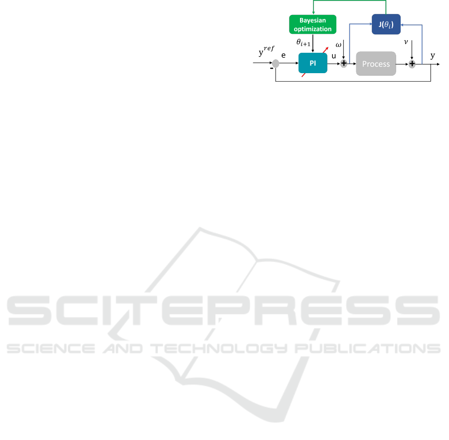
The auto-tuning of a PI controller in a real plant is the

focus of this paper. A simple scheme of the PI con-

troller is shown in Fig. 2. The signal y

re f

is the refer-

ence or set point to be tracked. u and y are respectively

the input and output of the process. ω represents the

process perturbation, and ν denotes the measurement

noise. e = y

re f

− y is the tracking error.

Figure 1: PI controller.

The PI controller has the following structure:

e(t)+ K

e(t)dt (1)

where K

and K

represents the proportional and inte-

gral gains. An anti-windup measure is also considered

to ensure the actuator constraints.

To tune the controller gains (K

and K

), we need

to deﬁne a cost function based on the desired track-

ing performance of the PI controller (i.e., overshoot,

settling time, integral absolute error (IAE), integral

ICINCO 2025 - 22nd International Conference on Informatics in Control, Automation and Robotics

236

time absolute error (ITAE), etc.). In this paper, a lin-

ear combination of commonly used control key per-

formance indicators (KPIs): settling time, overshoot,

and IAE is deﬁned in the following equations:

Osh(θ) + a

St(θ) + a

IAE(θ) (2)

where a

,i = 1 : 3, are known and constant weights. θ

is a vector that contains the control parameters. Osh

and St are the overshoot and settling time, respec-

tively. IAE represents the Integrated Absolute Error

and is given by: IAE =

∞

| e(t) | dt.

This speciﬁc set of KPIs is chosen to cover typ-

ical dynamic responses of interest, such as settling

when changing references (settling time), minimizing

error to reference (IAE), and limiting overshoot, as

many thermal plants are particularly sensitive to very

low overshoot. The weights are selected to provide

a quantiﬁable performance from the step response,

based on qualitative evaluation by a plant expert.

The auto-tuning PI controller is now formulated

as a black-box multi-objective optimization problem

given by:

min

s.t. θ = [K

],θ

≤ θ ≤ θ

l p

(3)

and θ

l p

are respectively the upper and lower

bounds of each element in the vector θ. The primary

objective at this juncture is to ﬁnd the optimal solution

for the challenging optimization problem (3). Given

the absence of a closed-form expression for the ob-

jective function and its expensive evaluation (or sam-

pling), the Bayesian optimization approach emerges

as the most appropriate choice. The costly nature of

objective function evaluation is attributed to the in-

tended tuning on the actual process during the com-

missioning phase. In Figure 2, we illustrate the ex-

ecution of the optimization framework using the BO

approach. Due to space limitations, we refrain from

providing in-depth technical details about the BO op-

timization approach. Readers seeking a comprehen-

sive explanation are encouraged to refer to the rele-

vant literature, such as (Garnett, 2023), for a more

detailed understanding. Unfortunately, even though

the BO approach is a promising technique, its perfor-

mance faces efﬁciency challenges due to the limited

number of conﬁguration evaluations possible within

a constrained budget. Moreover, incorporating avail-

able historical data is not straightforward. This prob-

lem is very challenging, mainly due to the difﬁculties

in extracting source knowledge from available data

and aggregating and transferring this knowledge to

the new target domain. In the literature, this prob-

lem is primarily addressed in hyper-parameter opti-

mization, with some interesting solutions proposed.

Figure 2: BO-based PI controller auto-tuning, where i indi-

cates a closed-loop experiment with controller parameters

For instance, (Perrone et al., 2019) suggested limiting

the search space of the optimized process (target task)

to sub-regions extracted from historical data. In (Li

et al., 2022), a different two-phase transfer learning

framework for automatic hyper-parameter optimiza-

tion is proposed, which can simultaneously handle the

complementary nature among source tasks and dy-

namics during knowledge aggregation. This solution

is adopted in this paper to accelerate the Bayesian op-

timization framework, and the approach will be pre-

sented in the next section.

3 ACCELERATE THE PI TUNING

IN COMMISSIONING PHASE

USING TRANSFER LEARNING

In this section, we explain how to use transfer learn-

ing technique for accelerating the auto-tuning of a

PI controller in the commissioning phase. Without

loss of generality, it is assumed that historical data is

available or can be generated from existing simulation

models. Indeed, data can be generated from variants

of the same model by altering the values of unknown

or uncertain parameters. For instance, if you have a

simulation model with several parameters whose ex-

act values are not known, you can create different

scenarios by systematically varying these parameters

within plausible ranges. This process allows you to

explore a wide range of possible outcomes and gen-

erate a diverse datasets. Additionally, this approach

provides a richer set of data that captures the variabil-

ity and uncertainty inherent in real process.

The transfer learning is conducted using the ap-

proach proposed by (Li et al., 2022) and illustrated

in Fig. 3. This approach addresses two main chal-

lenges. The ﬁrst challenge is how to tackle the

complementary nature among source tasks and ex-

tract source knowledge cooperatively. To solve this,

TransBO builds a source surrogate by combining base

surrogates from multiple source tasks using learned

weights. This phase ensures that the complementary

Enhancing PI Tuning for Plant Commissioning Using Transfer Learning and Bayesian Optimization

237

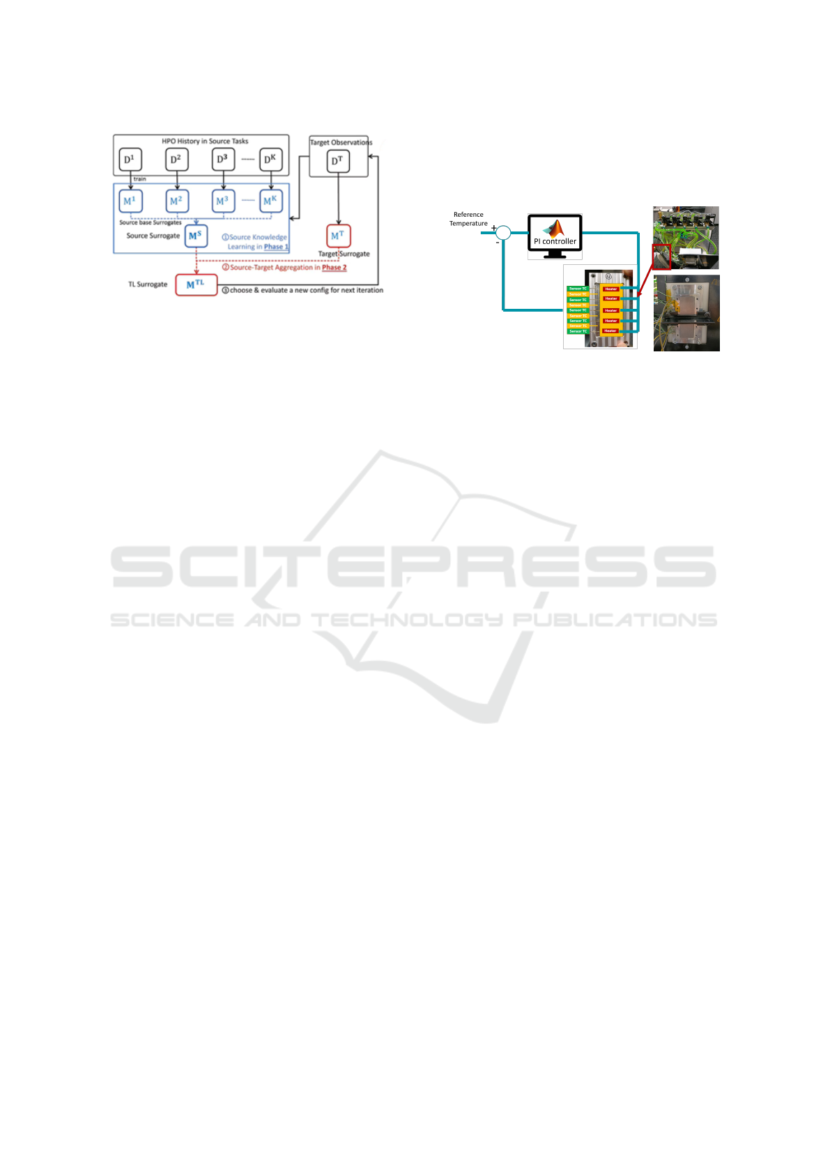
Figure 3: Two-Phase Transfer Learning Framework (Li

et al., 2022).

nature of different source tasks is utilized effectively.

The second challenge is how to handle knowledge

transfer as more target measurements become avail-

able. This is solved in a second phase, where the

source surrogate is combined with the target surro-

gate to form the ﬁnal transfer learning surrogate. This

combination is done in an adaptive manner, allowing

the framework to balance between source and target

knowledge dynamically. TransBO learns the weights

for combining surrogates by solving constrained op-

timization problems with a differentiable ranking loss

function. This principled approach ensures that the

knowledge transfer is both effective and adaptive,

leading to better performance with fewer evaluations.

To maximize the generalization ability of the transfer

learning surrogate, TransBO uses cross-validation to

learn the aggregation weights. This helps in prevent-

ing overﬁtting and ensures that the surrogate model

remains robust.

4 AUTO-TUNING PI

CONTROLLER FOR A

THERMAL PLANT

4.1 Set-Up

As a practical use case a thermal plant setup has been

used to demonstrate and validate the tuning meth-

ods in a realistic environment, resembling on one end

cooling of powertrain components, and on the other

typical industrial plastic curing, and drying applica-

tions.

The setup shown in ﬁgure 4, consists of an alu-

minum plate split into ﬁve distinct zones each heated

by a cartridge heater of 113W, which is in turn pow-

ered by a solid-state relay (SSR) applying a PWM 0-

220 V DC. Next to the heating, each of the zones is

also actively cooled on the back end by liquid cooling

through a cooling channel using water-glycol. The

valves on the entry of each of the ﬁve cooling chan-

nels allows for opening and closing, while the speed

controllable pump, enables ﬂow control through the

opened channels.

Figure 4: Experimental setup: thermal plant.

The thermal measurements are recorded by a to-

tal of nine (9) thermocouples, glued into each of the

ﬁve aluminum zones, but also the boundary between

each two zones. The thermocouples are calibrated to

+-1C accuracy. The ﬂuid temperature are measured

by Pt100 sensors on input/output coolant lines. Addi-

tionally, pressure across the setup and the ﬂow rate of

the water glycol are measured, both for safety and for

validation purposes.

All the controls and measurements are interfaced

to a Beckhoff I/O stack connected over EtherCAT to

a Xenomai Triphase real-time target. The base sam-

pling time of the control loop is Ts = 1ms while the

sensor measurements are logged at Tmeas = 100ms,

which is deemed sufﬁcient for a rather slow thermal

process. This allows for rapid prototyping of control

code in Simulink and easy integration to test environ-

ment in MATLAB.

4.2 Thermal Plant Model

As mentioned in 3, a model is needed for calculating

the initial condition and the upper and lower bounds

of the controller gains before running the BO with

the real plant in the commissioning phase. The used

model is a physics-based white box model with dy-

namic of heat dissipation, convection losses and heat

exchange between different components. This plant

model is excited by multiple disturbances and evalu-

ated in a closed loop simulation with a feedback con-

troller (PI).

4.2.1 Thermal Model Assumptions

The thermal plant model is a second order model,

consisting of two connected metal masses. The model

buildup and numerical evaluation was performed in

python. The thermal model under investigation in-

cludes the main modes of heat exchange between and

ICINCO 2025 - 22nd International Conference on Informatics in Control, Automation and Robotics

238

within the components:

• One block, ”mass 1 (copper)” is heated internally,

through direct heat injection. this is equivalent to

heating by an electric resistor inserted in this vol-

ume.

• A second block, ”mass 2 (aluminium)” is cooled

internally, driven by a cooling temperature and

given transfer area and heat transfer coefﬁcient.

This is equivalent to cooling through a glycol-

water mixture, circulating at high throughput rate

through pipes in the volume).

• The two metal blocks (aluminium and copper)

are connected and do exchange (when at differ-

ent temperatures) heat by conduction through an

area of contact.

• Also, both blocks are in contact with surrounding

air and lose or gain thermal energy through con-

vection.

4.2.2 Model Structure

The model structure is as follows:

Two states are deﬁned, representing the bulk cop-

per temperature (T

node,Cu

) and the bulk aluminum

temperature (T

node,Alu

). Heat injection and loss

(through cooling and resistive heating) and heat losses

or gains are injected directly into these states.

The node temperatures are updated every time

step using a backward Euler scheme, with the com-

bined energy inputs of each of the heat losses and

gains.

The heat gains and losses from heating dT

and

cooling dT

are a deﬁned as:

H,t−1→t

= Q

/m/cp ∗ dt

and

C,t−1→t

= Q

/m/cp ∗ dt

whereby the heat gain Q

is driven directly by the

PI-controller, and

= −(h

alu,C

∗ A

alu,C

∗U

alu,C

∗ (T

C,t

− T

alu

) ∗ dt)

As the two blocks have a different temperature and

are physically connected along area A, a heat ﬂow

through conduction dT

othermat

will be induced. The

ﬂux q

Alu,Cu

is a function of their respective temper-

atures and distance of bulk temperature nodes. The

joint temperature is deﬁned as a function of to the per-

pendicular distances between the cooling and heating

nodes and the joint:

joint,t

∗ k

alu

∗ L

node,alu

+ T

Alu

∗ k

∗ L

node,cu

alu

∗ L

node,alu

+ k

∗ L

node,cu

The resulting heat ﬂow Q

Alu,Cu

depends on the

contact area and mass of the materials(s):

alu,cu

∗ q

Alu,Cu

= −A

alu,cu

∗ q

Cu,Alu

= (T

node,Alu

− T

joint,t

) ∗ cp

alu

∗ m

alu

∗ dt

On the other hand, heat loss to the environment

is modelled using conduction through a given surface

air

with thermal transmittance U

air

and T

ext

the exte-

rior temperature:

air,t−1→t

= −(T

node,t−1

−T

ext

)∗A

air

∗U

air

/m/cp∗dt

The numerical values for the model parame-

ters and initial state are summarized in Table 1 of

(Boulkroune et al., 2024). For this analysis, these val-

ues are primarily held constant; however, they can be

made variable, and noise can be introduced into the

disturbance, input, and output signals.

4.3 Results and Benchmarking

Experiment description follows (see Figure 5). Each

experiment lasts for a total of 380 seconds. It begins

with a warmup to 25C for min relying on a well-tuned

PI parameters (this ensures consistency in compari-

son between different runs), followed by a bumpless

transfer of control parameters to the tested PI combi-

nation, so that the sudden change in integrator param-

eter does not create a large step in the output of the

controller. Finally, a step reference is applied at 140

seconds and is recorded for length of 120 seconds.

The experiment ends with a cool-down period of 120

seconds back to below 25C so that the next experi-

ment can be started. For the computation of the ob-

jective function, exclusively the data within the time

interval of 140 to 260 seconds is considered.

The description of how the experiments were re-

alized is illustrated in Figure 5. Each experiment lasts

for a total of 380 seconds. It begins with a warm-

up to 25°C for a few minutes, relying on well-tuned

PI parameters (this ensures consistency in compari-

son between different runs). This is followed by a

bump less transfer of control parameters to the tested

PI combination, so that the sudden change in the in-

tegrator parameter does not create a large step in the

output of the controller. Finally, a step reference is

applied at 140 seconds and is recorded for a length of

120 seconds. The experiment ends with a cool-down

period of 120 seconds back to below 25°C so that the

next experiment can be started. For the computation

of the objective function, exclusively the data within

the time interval of 140 to 260 seconds is considered.

In a previous study, we conducted a total of 256

experimental runs based on the procedure explained

earlier. Due to the signiﬁcant time and ﬁnancial costs

Enhancing PI Tuning for Plant Commissioning Using Transfer Learning and Bayesian Optimization

239

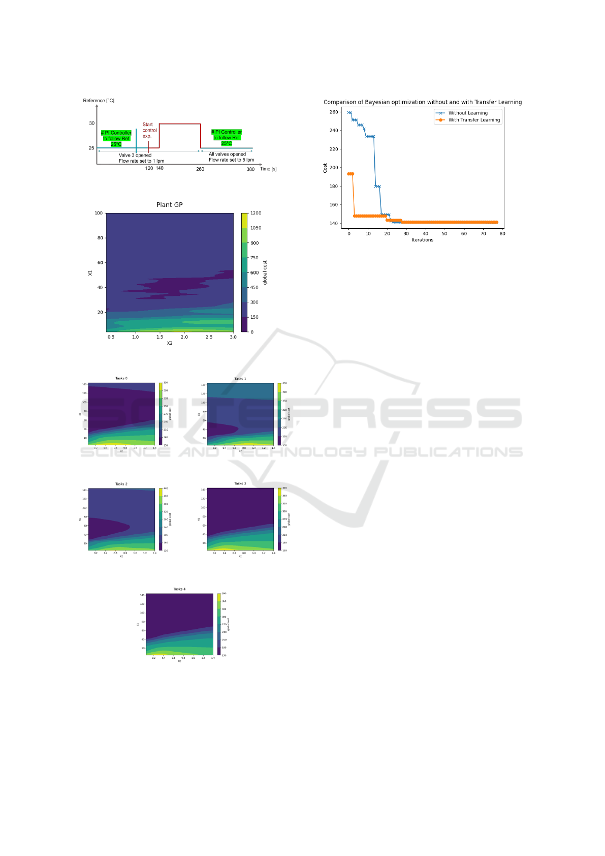
Figure 5: Experiment description.

Figure 6: Cost heat map.

(a) m

= 0.5 ∗ ˆm

node,cu

(b) m

= 0.75 ∗ ˆm

node,cu

= 1 ∗ ˆm

node,cu

(d) m

= 1.25 ∗ ˆm

node,cu

(e) m

= 1.75 ∗ ˆm

node,cu

Figure 7: Data generated from different thermal model vari-

ants.

Figure 8: Comparison of BO without and with transfer

learning.

associated with repeating these tests, we opted to uti-

lize the collected data by ﬁtting it to a Gaussian Pro-

cess (GP) model. This model is then used as a sur-

rogate for the actual plant, thereby avoiding the need

for further costly and time-consuming experiments.

The cost heat map of the collected data is presented

in Figure 6. On the other hand, to compensate for the

lack of historical data, the presented thermal model

will be used for generating data. First, the unknown

parameters in the thermal model are identiﬁed using

a Bayesian approach. The main idea is to enhance

the model prediction capability by trying to iden-

tify as accurately as possible the unknown parame-

ters. It is both reasonable and non-limiting to assume

that the model parameters are identiﬁable. Alterna-

tively, it may be feasible to downsize the model, re-

taining only the identiﬁable sub-system whenever ap-

plicable. At this stage, acquiring experimental data

is essential to understand the true dynamics of the

plant and only one single experiment is required. It

is worth noting that the objective is not to get an

exceedingly precise model, but rather to achieve a

model of satisfactory accuracy, suitable for generat-

ing historical data from the model variants. These

variants can be obtained from the identiﬁed model

by varying the values of the identiﬁed unknown pa-

rameters within a speciﬁed ranges. Other alternatives,

if you have a simulation model with several parame-

ters whose exact values are not known, you can cre-

ate different scenarios by systematically varying these

parameters within plausible ranges. In our study,

the ﬁrst approach is used. The mass of the cupper

(i.e,m

node,cu

) is the only unknown parameters identi-

ﬁed and ﬁve (5) simulation data are obtained using

the values : 0.5 ∗ ˆm

node,cu

, 0.75 ∗ ˆm

node,cu

, 1 ∗ ˆm

node,cu

1.25 ∗ ˆm

node,cu

and 1.75 ∗ ˆm

node,cu

, where ˆm

node,cu

the identiﬁed parameter ( ˆm

node,cu

= 0.8262). The ob-

tained cost heat maps are presented in ﬁgure 7. This

ICINCO 2025 - 22nd International Conference on Informatics in Control, Automation and Robotics

240

data will be used as historical data for transfer learn-

ing purposes. As we can see, this data exhibits dif-

ferent optimal regions depending on the mass of the

cupper.

Instead of conducting a comparison with manual

tuning, we opted to employ another optimization ap-

proach: Bayesian Optimization (BO) without transfer

learning. For both BO techniques (with and without

transfer learning), we used the developed tool ’Open-

box’ by (Jiang et al., 2024), which is publicly avail-

able at

. For BO without transfer learning, the default

conﬁguration was used (i.e, surrogate type =

′

initial runs = 1, init strategy =

′

de f ault

′

). For

BO with transfer learning, the following conﬁgura-

tion was used: initial trials = 5, init strategy =

′

de f ault

′

, surrogate type =

′

tlbo topov3 gp

′

acq optimizer type =

′

random scipy

′

. The con-

sidered ranges (upper and lower bounds) for the

proportional gain (KP) and integral gain (KI) were

deﬁned as [4,100] and [0.1,3], respectively. The ini-

tial guess is chosen as K

= 89.96 and K

= 0.2003

for both approaches.

The comparison results between BO with and

without transfer learning are shown in Figure 8. The

x-axis represents the number of iterations, while the

y-axis represents the cost. Evidently, the BO with

transfer learning achieves a convergence rate that is

76% faster than BO without transfer learning. A

notable performance obtained even considering the

moderate model prediction quality. There is poten-

tial for further enhancement in this percentage if ad-

ditional efforts are invested in reﬁning the model pre-

dictions.To ensure a fair comparison between the two

optimization algorithms, it is advisable to run them

with several initial guess points. This approach helps

to mitigate the inﬂuence of any single starting point

on the optimization results, providing a more compre-

hensive evaluation of each algorithm’s performance.

By using multiple initial guesses, we can better as-

sess the robustness and effectiveness of the algorithms

across a broader range of scenarios. Due to time con-

straints, this will be done in the future, together with

direct application to the real thermal plant.

5 CONCLUSION

In this study, we proposed a novel approach to ac-

celerate the auto-tuning of PI controllers during the

commissioning phase. By combining transfer learn-

ing and Bayesian optimization, we aimed to minimize

the number of iterations needed to reach the opti-

mal solution. Transfer learning was utilized to extract

https://github.com/PKU-DAIR/open-box

valuable insights from historical data obtained from a

simulation model. The effectiveness of our approach

was demonstrated through its application to a thermal

plant, signiﬁcantly reducing the number of iterations

required to achieve the optimizer’s optimal solution.

ACKNOWLEDGMENT

The research was supported by VLAIO under the

project HBC.2022.0052 Tupic-ICON performed in

Flanders Make.

REFERENCES

Aidan, O. (2006). Handbook of PI and PID Controller Tun-

ing Rules. Imperial College Press.

Bazanella, A. S., Campestrini, L., and Eckhard, D. (2011).

Data-driven controller design: The h

approach.

Springer Science and Business Media.

Boulkroune, B., Jordens, X., Mrak, B., Verhelst, J., De-

praetere, B., Meskens, J., and Bovijn, P. (2024). En-

hancing pi tuning in plant commissioning through

bayesian optimization. In ECC 2024, page

3220–3225.

Boyd, S., Hast, M., and

Astr

om, K. (2016). Mimo pid tun-

ing via iterated lmi restriction. Int. J. Robust Nonlin-

ear Control, 26:1718–1731.

Campi, M., Lecchini, A., and Savaresi, S. (2002). Vir-

tual reference feedback tuning: A direct method

for the design of feedback controllers. Automatica,

38(8):1337–1346.

Doerr, A., Nguyen-Tuong, D., Marco, A., Schaal, S., and

Trimpe, S. (2017). Model-based policy search for au-

tomatic tuning of multivariate pid controllers. arXiv.

arXiv:1703.02899.

Fujimoto, Y., Sato, H., and Nagahara, M. (2023). Controller

tuning with bayesian optimization and its accelera-

tion: Concept and experimental validation. Asian J

Control, 25:2408–2414.

Garnett, R. (2023). Bayesian Optimization. Cambridge

University Press, Cambridge, 1st edition.

Gevers, M. (2002). Modelling, identiﬁcation and control,

page 3–16. Springer-Verlag.

Hjalmarsson, H. (1998). Control of nonlinear systems using

iterative feedback tuning. In Proceedings of the 1998

American Control Conference, page 2083–2087.

Ho, W., Hong, Y., Hansson, A., Hjalmarsson, H., and Deng,

J. (2003). Relay autotuning of pid controllers using

iterative feedback tuning. Automatica, 39(1):149–57.

Jiang, H., Shen, Y., Li, Y., Xu, B., Du, S., Zhang, W., Zhang,

C., and Cui, B. (2024). Openbox: A python toolkit for

generalized black-box optimization. Journal of Ma-

chine Learning Research, 25(120):1–11.

Kaneko, O., Soma, S., and Fujii, T. (2005). A new approach

to parameter tuning of controllers by using one-shot

Enhancing PI Tuning for Plant Commissioning Using Transfer Learning and Bayesian Optimization

241

experimental data - a proposal of ﬁctitious reference

iterative tuning. In 16th IFAC World Congress, vol-

ume 38, page 626–631.

Kinoshita, T. and Yamamoto, T. (2018). Design of a data-

oriented pid controller for a two degree of freedom

control system. In 3rd IFAC Conference on Advances

in Proportional-Integral-Derivative Control PID, vol-

ume 51, page 412–415.

Li, Y., Shen, Y., Jiang, H., Zhang, W., Yang, Z., Zhang, C.,

and Cui, B. (2022). Transbo: Hyperparameter opti-

mization via two-phase transfer learning. In SIGKDD

2022.

Liuping, W. (2017). Automatic tuning of pid controllers

using frequency sampling ﬁlters. IET Control Theory

Appl, 11(7):985–95.

Lu, H., Shu-yuan, W., and Sheng-nan, L. (2017). Study and

simulation of permanent magnet synchronous motors

based on neuron self-adaptive pid. In 2017 Chinese

Automation Congress (CAC), page 2668–2672, Jinan,

China.

Perrone, V., Shen, H., Seeger, M., Archambeau, C., and Je-

natton, R. (2019). Learning search spaces for bayesian

optimization: Another view of hyperparameter trans-

fer learning. In Advances in Neural Information Pro-

cessing Systems, volume 32.

Reynoso-Meza, G., Sanchez, H. S., Blasco, X., and Vi-

lanova, R. (2014). Reliability based multiobjective

optimization design procedure for pi controller tuning.

In 19th World Congress, page 10263–10268.

Sanchis, R. and Pe

narrocha-Al

os, I. (2022). A new method

for experimental tuning of pi controllers based on the

step response. ISA Trans., 128:329–342.

Shipman, W. (2021). Learning to tune a class of con-

trollers with deep reinforcement learning. Minerals,

11(9):989.

ICINCO 2025 - 22nd International Conference on Informatics in Control, Automation and Robotics

242