Wind Farm Power Prediction Using a Machine Learning Surrogate

Model from a First-Principles Simulation Model

Sebastian E. Pralong

, Samuel Martínez-Gutiérrez

, Dan E. Kröhling

, Alejandro Merino

Gonzalo E. Alvarez

, Daniel Sarabia

and Ernesto C. Martínez

Instituto de Desarrollo y Diseño INGAR (CONICET/UTN), Avellaneda 3657, S3002GJC, Santa Fe, Argentina

Departarmento de Digitalicación, Avda. Cantabria s/n., Universidad de Burgos, 09006 Burgos, Spain

Keywords: Renewable Energy, Machine Learning, Real-Time Forecasting, Energy Management.

Abstract: Reliable forecasting of wind farm power generation is essential for ensuring seamless grid integration and

optimizing energy management strategies. This paper presents an integrated framework combining a first-

principles simulation model of wind turbines as a data source for machine learning techniques to forecast

wind farm power output. The simulation model accounts for wind speed, direction, temperature, and other

climate variables, and is computationally intensive due to the need to account for the dynamics of each turbine

operation, the wake effects, etc. To diminish the computational cost, this work introduces a surrogate Gaussian

Processes (GPs) model that approximates the complex simulation model to provide predictions of both the

mean and variance of power generation. To forecast future climate conditions, we employ a NARX (Nonlinear

Autoregressive with Exogenous Inputs) neural network trained on historical data to account for wind speed,

direction, and atmospheric conditions for the next two hours. The NARX model forecasts and the GPs

predictions enable fast and accurate real-time forecasting of power generation for the entire wind farm. This

approach significantly reduces computational times from hours to seconds while maintaining high accuracy,

offering a scalable and efficient solution for real-time wind farm power prediction and online optimization.

1 INTRODUCTION

Wind energy has become a pillar of renewable energy

systems and has played an integral part in

international efforts to decrease carbon emissions and

attain sustainable energy objectives (Ali & Meo,

2024). The integration of wind farms into grids is not

an easy task due to the intrinsic variability of wind

and its effect on output. Predicting the output of wind

farms accurately and in a timely manner is crucial for

optimal grid management, scheduling energy, and

operational optimization (Landberg, 1999). The

conventional first-principles simulation models that

capture the intricate nature of wind turbine operations

and environmental interactions are highly accurate

https://orcid.org/0009-0007-5797-5246

https://orcid.org/0000-0003-1790-9344

https://orcid.org/0000-0002-3115-1800

https://orcid.org/0000-0002-8301-7195

https://orcid.org/0000-0003-1602-8051

https://orcid.org/0000-0001-7802-3542

https://orcid.org/0000-0002-2622-1579

but have high computational expense and take hours

for a single simulation of a single instance (Douvi &

Douvi, 2023). Their use for real-time prediction and

online optimization is therefore unfeasible due to high

computational times. New developments in machine

learning have provided an opportunity for solving this

issue by creating surrogate models that are

approximations of expensive simulations but with a

minute fraction of the computational demand.

In this article, an original framework is presented

that couples a control oriented first-principles

simulation model with machine learning methods for

rapid and accurate prediction of wind farm power

output.

This paper employs modular, first-principles-

Pralong, S. E., Martínez-Gutiérrez, S., Kröhling, D. E., Merino, A., Alvarez, G. E., Sarabia, D. and Martínez, E. C.

Wind Farm Power Prediction Using a Machine Learning Surrogate Model from a First-Principles Simulation Model.

DOI: 10.5220/0013709700003982

Paper published under CC license (CC BY-NC-ND 4.0)

In Proceedings of the 22nd International Conference on Informatics in Control, Automation and Robotics (ICINCO 2025) - Volume 1, pages 417-424

ISBN: 978-989-758-770-2; ISSN: 2184-2809

417

based models in EcosimPro (EA International, 2024),

balancing accuracy and simplicity. These models

simulate turbine power output with minimal

parameters, omitting detailed aerodynamic or

electrical submodels. Integrated controls manage

turbine startup, shutdown, rotor orientation, and

power output, with wind farms modeled to include

wake interactions but not energy transport. Compared

to tools like OpenFAST or SOWFA, EcosimPro

models are suited for control-oriented and system-

level simulations.

The simulator’s key advantage is generating high-

quality synthetic data for data-driven algorithms.

Real-world data is often limited by privacy,

proprietary restrictions, or sensor issues (Li et al.,

2020). The simulator explores all input combinations

(wind speed, direction, control modes), creating

comprehensive datasets that prevent poor

generalization or hallucinations in neural networks,

supporting robust AI model development for wind

farm control and optimization.

We employ a Gaussian Process (GP) surrogate

model to approximate the computationally intensive

simulation model, predicting mean and variance of

wind farm power output based on environmental

variables like wind speed, direction, and air pressure.

For climate forecasts, a Nonlinear Autoregressive

with Exogenous Inputs (NARX) neural network

estimates wind and atmospheric conditions for the

next two hours, offering advantages over public

forecast products due to better adaptation to site-

specific characteristics and lower latency. Integrating

NARX forecasts with the GP model enables fast,

accurate power predictions in seconds, as detailed in

the methodology.

The main aim of the proposed approach is the

establishment of an efficient and scalable framework

for real-time prediction of wind farm power. Through

a combination of a GP surrogate model and a NARX

neural network, we can achieve high accuracy by

utilizing data generated from first-principles

simulations while minimizing computational costs by

orders of magnitude. This makes it applicable in real-

time grid integration, energy management, and online

optimization problems, and provides a robust solution

for improving wind farm operating efficiency.

2 METHODOLOGY

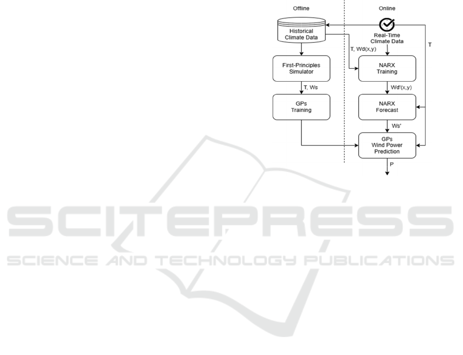
This study employs a two-stage, offline/online

approach to achieve efficient and accurate wind farm

power prediction as it is shown in Figure 1. During

the offline stage, a first-principles simulation model

is used to generate power output data for a wind farm

under varying climate and wind conditions,

accounting for turbine dynamics and wake effects.

These simulations provide the foundational dataset

for training a Gaussian Processes (GPs) surrogate

model, which approximates the computationally

intensive simulation model while delivering rapid

predictions with uncertainty quantification.

Figure 1: Methodological approach.

During the online stage, as real-time data is

acquired, a Nonlinear Autoregressive with

Exogenous Inputs (NARX) neural network is trained

on historical meteorological data to forecast wind

speed, direction, and atmospheric variables over short

time horizons. The integration of the NARX-based

forecasts with the GP model allows for fast, reliable

power output estimations, bridging the gap between

accuracy and computational efficiency. Within this

methodology, synthetic data can be substituted with

real historical data.

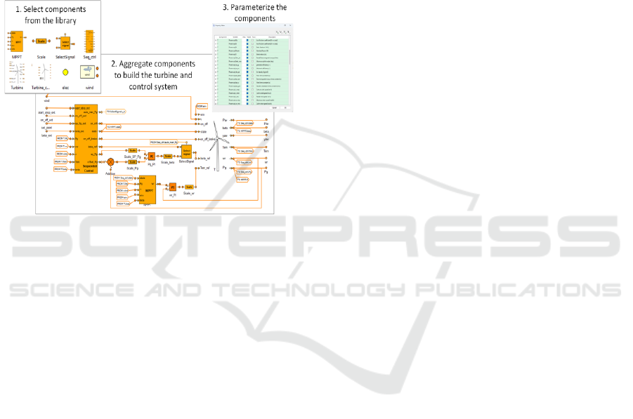
2.1 First-Principles Simulator

The simulator used as a data source for this work has

been developed as a modular library of dynamic

models in the EcosimPro platform. The simulator is

designed to bridge the gap between highly detailed

tools such as OpenFAST (OpenFAST, 2024) and

low-complexity solutions like the WindPowerPlants

Modelica library (Eberhart, 2015), offering a balance

between modeling accuracy and computational

efficiency. Its main purpose is to support control

design and operational optimization of wind farms,

enabling fast execution on standard computing

systems. The structure can be observed in Figure 2.

The wind turbine model is based on a two-mass

mechanical representation, capturing the torsional

ICINCO 2025 - 22nd International Conference on Informatics in Control, Automation and Robotics

418

dynamics between the rotor and the generator through

a flexible shaft. The model includes local control

systems for rotor speed and generated power,

implemented with Proportional-Integral (PI)

controllers. Turbines are assumed to be of the doubly-

fed induction generator (DFIG) type, and the control

logic accommodates both pitch regulation and rotor

speed tracking to implement maximum power point

tracking (MPPT) strategies. Besides power

generation control, the overall control system

implemented includes turbine startup and shutdown

and rotor orientation to current wind direction.

Figure 2: Structure of the EcosimPro Platform.

In addition to individual turbine dynamics, the

simulator accounts for wake effects using the multiple

shadow Jensen/Katic model. This approach estimates

the wind speed reduction at each turbine due to

upstream turbines, considering thrust coefficients,

and supporting the modeling of partial wake overlap.

This enables a realistic prediction of power losses due

to turbine interaction within the farm.

At the wind farm level, the simulator implements

several centralized control strategies compatible with

the local control systems, with built-in mechanisms

for safe mode switching and fault handling.

2.2 Gaussian Process

Gaussian Processes (GPs) (Rasmussen & Williams,

2019) are machine learning models used for

regression tasks that provide predictions and

confidence intervals. One of their advantages is the

ability to model complex interactions between

variables without explicit parameterization. Thanks

to this flexibility, GPs can adapt to different types of

data. Equation 1 shows the general form of a GP.

𝑓(𝑥) ∼ 𝐺𝑃 (𝑚(𝑥), 𝑘(𝑥, 𝑥′)) (1)

where the mean function is 𝑚(𝑥) (usually set to

0), and 𝑘(𝑥, 𝑥′) is the covariance function or kernel

between each pair of elements. In this work, each

element is a vector comprising two variables at each

point in time: wind speed and temperature. These

variables were selected over others due to their higher

correlation with wind power generation, as it was

determined from historical data analysis (see Section

4.2). Moreover, the GP is a multivariate GP, as two

variables are considered.

The kernel is used to define the similarity between

two elements 𝑥 and 𝑥′. In this work, the GP is a sum

of two kernels. The first is a Matérn kernel

(Pedregosa et al., 2011) with two hyperparameters:

the length scale 𝑙, which is set to 5, and an additional

parameter 𝜈 that controls the smoothness of the

resulting function, which is set to 1.5. The second is

a constant kernel that allows for incorporating the

mean value of the measurements. The kernel and

hyperparameters values were selected after

conducting a hyperparameter optimization.

2.3 NARX Neural Network

Nonlinear Autoregressive Network with Exogenous

Inputs (NARX) (Siegelmann et al., 1997) is a type of

recurrent neural network designed to model dynamic

systems whose evolution depends on both their past

values and external inputs. This architecture is

particularly suitable for tasks such as time series

prediction and modelling of non-linear dynamic

systems. The main advantage of NARX networks lies

in their ability to capture complex temporal

relationships with a trainable and efficient

architecture. These networks are widely used in

modelling and prediction in areas such as renewable

energy, economics, control engineering and fault

diagnosis (Hansda & Murmu, 2023).

Mathematically, a NARX network models the

output y(t) as a function of a series of past values of

the output itself and one or more external inputs x(t),

according to the following structure:

𝑦(𝑡) =𝐹(𝑦(𝑡−1),..,𝑦(𝑡−𝑑𝑦);

(2)

𝑥(𝑡−1),..,𝑥(𝑡−𝑑𝑥))

where y(t) is the system output at time t, x(t) is the

exogenous input to the system, dy, dx are the output

and input delays, respectively, and F is the nonlinear

function approximated by the network.

There are two main modes of operation in NARX

neural networks (Rahman et al., 2022). Open-loop

mode: during training, past actual values of the output

are used as feedback. Closed-loop mode: during

simulation or future prediction, the network is fed

Wind Farm Power Prediction Using a Machine Learning Surrogate Model from a First-Principles Simulation Model

419

with its own estimated outputs, allowing long-term

behavior to be predicted without relying on actual

future data.

2.3.1 Neural Network Structure

The dataset is provided by a nearby weather station in

table format and includes columns representing

meteorological variables temperature and wind

components for which data are taken every 30

minutes. It is chosen to work with the perpendicular

wind components instead of wind direction and

modulus (wind speed) to avoid problems of

continuity in angles and training errors. For example:

an angle of 0º and 350º are numerically distant but

physically not. To fit the data to a NARX neural

network, all values are normalized between 0 and 1.

This normalization is performed using the minimum

and maximum values per column, previously

extracted from the network configuration.

A NARX type neural network is created using the

narxnet function available in Matlab software

(Matlab, n/d). The network is set in open-loop

training mode, which allows using the real data

passed as feedback during the training phase.

The network structure has component values to be

defined. Input layer: receives the past values of both

the output variable and the exogenous variables. A

delay of 4 time steps is used, so that the inputs at

instant t correspond to the values at t-1, t-2, t-3 and t-

4. Hidden layer: Composed of 10 neurons, each of

which employs the sigmoidal tangent transfer

function (tansig). This non-linear function allows the

network to model complex, non-linear relationships

between input and output variables. Output layer: It

uses a linear transfer function (purelin) that allows

predictions to cover the entire real range of values,

which is indispensable for continuous physical

variables such as wind speed. The network was

trained using the Levenberg-Marquardt

backpropagation algorithm, which is particularly

effective for problems with a relatively small number

of parameters and well-conditioned inputs, which

matches the characteristics of our experimental setup.

InputDelays = 1:4: uses the previous 4 values of the

inputs as the temporal context, in this case the two

wind components. FeedbackDelays = 1:4: uses the 4

previous values of the output as feedback.

2.3.2 Training, Prediction and Evaluation

The data are divided into the exogenous input time

series and output (target) which corresponds to the

endogenous feedback variables. The network is

trained (Figure 3) on the ‘W’ weights and ‘b’ biases

of both layers in open loop mode using the

normalized data. After training, the network is

converted to the closed-loop mode as shown in Figure

3, allowing it to predict autonomously, using its own

outputs as feedback. The prediction of future values

is then performed with this closed-loop network using

its own forecast data as input.

Figure 3: Changing the network from open to closed loop.

3 TEST CASE

As a case study, a mathematical model has been

developed for a fictitious park using the topology and

location of a real wind farm (El Valle-Valdenavarro)

in Navarra, Spain. Specifically, at geographical

coordinates: Latitude: 41°55’18.9’’ Longitude: -

1°25’46.9’’. The wind farm consists of 14 turbines

assumed to be of the NREL 5MW type and

parameterized according to the values available in

(Jonkman, J, et al 2009). The relative wind turbine

locations are shown in Figure 4.

One of the key aspects when simulating the

dynamic behavior of wind farms is the availability of

wind data at the specific locations where these farms

are situated. In this work, mesoscale data from the

New European Wind Atlas (NEWA, 2022) has been

used. This website provides meteorological data

every 30 minutes across the European Union for the

period from 2005 to 2018, obtained using the Weather

Research & Forecasting Model (WRF) (Witha et al.,

2019).

ICINCO 2025 - 22nd International Conference on Informatics in Control, Automation and Robotics

420

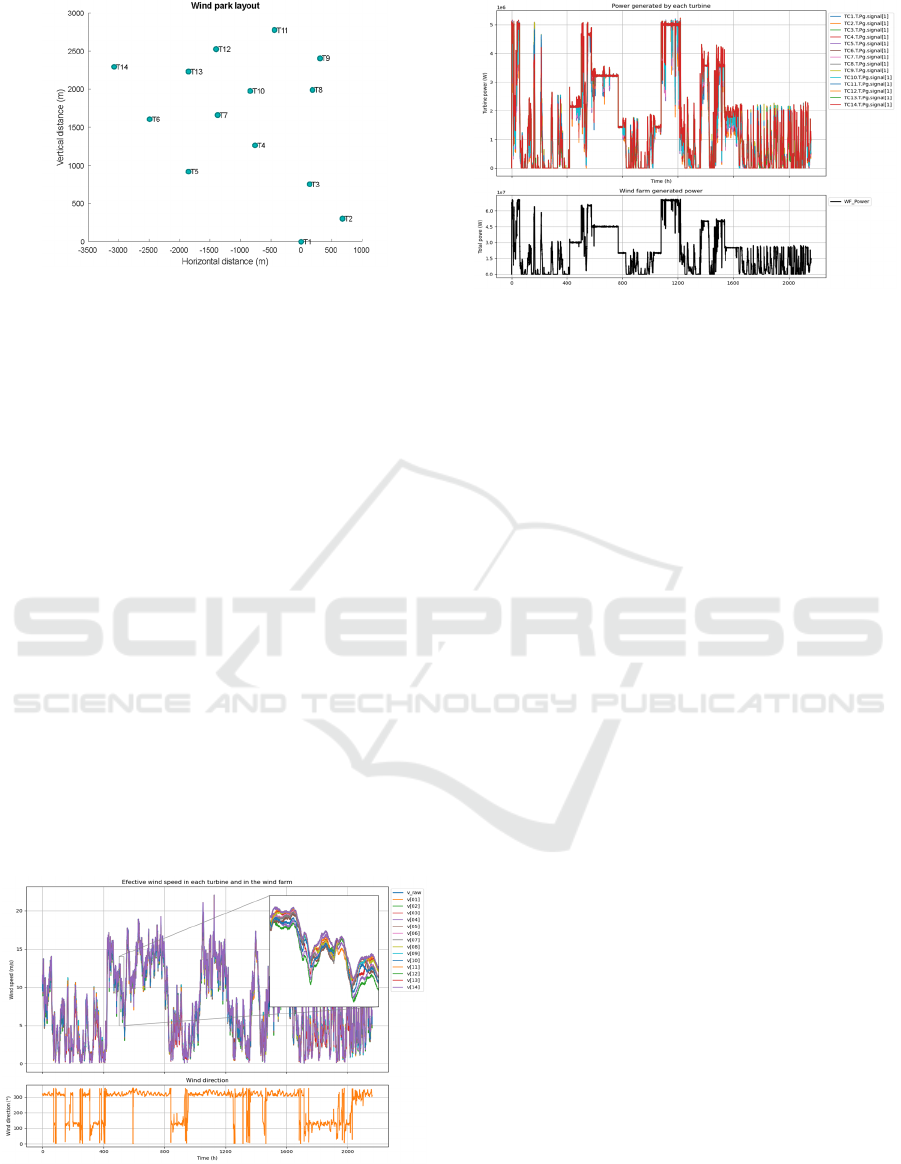
Figure 4: Layout of the turbines for the case study farm.

4 ANALYSIS OF RESULTS

4.1 Running on the Simulator

To generate the synthetic data needed to train the GP

model, the generation plant described in the previous

section was simulated over a three-month period,

with data recorded every 30 seconds. The wind farm

setpoint was set to 75 MW, exceeding the nominal

capacity of the wind farm (70 MW). As a result, the

turbines operated at their maximum possible output,

determined solely by wind conditions, effectively

running without curtailment and extracting the

maximum available power.

Some results of the simulation that are fed to the

GP model are presented next. Figure 5 and Figure 6

shows the undisturbed wind speed (v_raw) and the

effective wind speed at each turbine, estimated using

wake effect calculations, for a selected simulation

period. It can be observed that, depending on the wind

direction, the effective wind speed incident on each

turbine varies according to the wind farm layout.

Figure 5: Upper graph, wind speed data for each turbine.

Lower graph, wind direction data.

Figure 6: Upper graph, power generated by each turbine.

Lower graph, total power generated by the wind farm.

4.2 Gaussian Process Model Training

To train the GP, a number of variables are considered

as explanations for the total power generation of the

wind farm. The variables studied encompass: (a)

Total power generation, (b) Time of the day, (c) Air

density, (d) Temperature, (e) Atmospheric pressure,

(f) Wind speed, and (g) Wind direction. The predicted

variable is (a) Total power generation, while the

others are the possible predicting variables.

Figure 7 presents the correlation analysis between

variables. Based on the analysis, (f) Wind Speed and

(d) Temperature were selected as explanatory

variables due to their respective correlations of 0.95

and -0.33 with the target variable (a). Variable (c) Air

Density was excluded due to its high correlation with

(d) Temperature (-0.93), which was already included

as a predictor. Wind direction was not addressed in

this first trained model in order to simplify the

analysis and focus on the methodological aspects.

A multivariate GP model was developed to

predict wind farm power output using temperature

and wind speed as input features. The scope of this

study is limited to short-term (intraday) forecasting.

Wider temporal generalization may be crucial in

training over annual cycles and seasonal strategies.

Thus, the model is trained on data collected over a

period of three months, with measurements taken

every 30 minutes. Only two and a half months are

used as training data, resulting in a total of 3,600

training samples, while the remaining 15 days are

used for testing. The training took approximately 4

minutes. The R

score obtained by the GP is 0.9986.

Wind Farm Power Prediction Using a Machine Learning Surrogate Model from a First-Principles Simulation Model

421

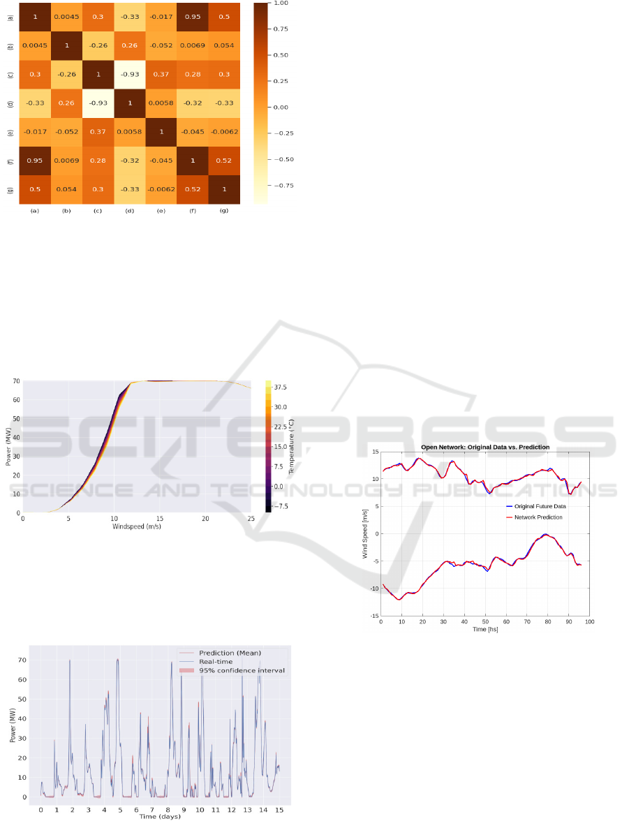
Figure 7: Correlation between variables.

Figure 8 provides a projected view of the fitted

GP, enabling comparison of the total power output

under different wind speed conditions. Temperature

is depicted using a color gradient, effectively

highlighting its impact on power generation. This

curve serves as a reliable foundation for modeling the

aggregate behavior of the wind farm.

Figure 8: Wind farm power under wind speed conditions.

Figure 9 presents the validation results over a 15-

day horizon, with predictions made at 60-second

intervals, resulting in 21,600 data points. The total

computation time for the forecast was 17 seconds.

Figure 9: GP validation results over a 15-day horizon.

4.3 Forecasting with NARX Networks

In order to evaluate the trained NARX network and

its forecasts, different points in time are taken within

the data series where the wind parameters in the wind

farm change substantially. The whole training

process is repeated for each new time selected.

Data is taken every 30 minutes using the last 100

measurements to train the network in each case.

Temperature is used as the exogenous input, and the

north-south and east-west wind components serve as

the endogenous outputs with feedback. The network

is trained in an open loop with the normalized time

series data and uses the 4 previous time values of the

inputs as historical context. The network is

configured as discussed in the methodology section

2.3.1 and 2.3.2. Figure 10 shows the open-loop

network fitted after training with 100 data of the

series for a particular time of the dataset. During

open-loop training, the mean square error (MSE) is

used, and a decrease in MSE is observed in the

training, validation, and test sets. This procedure is

repeated at different times during the training series.

The best validation performance is achieved in epoch

5. This value represents the optimal point of

generalization, thus avoiding overfitting. The training

time is approximately 8 seconds.

Figure 10: Open-loop model fitting.

The network model is switched from open-loop to

closed-loop to make the prediction for the next two

hours. The predictions of both wind components are

obtained denormalized as shown in Figure 11, where

both components (blue) are plotted with their

predictions (red) for the next 30, 60, 90 and 120

minutes. Using these data and predictions we can

obtain Figure 12 where the modulus and direction of

the velocity is represented, it can be observed how the

main variable that introduces error to the model is the

wind modulus (wind speed).

ICINCO 2025 - 22nd International Conference on Informatics in Control, Automation and Robotics

422

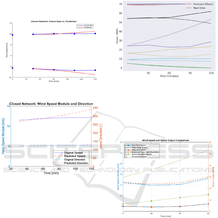
The normalized Root Mean Square Error (RMSE)

prediction error for the two-hour forecast is estimated

to average 11.19%.

Figure 11: Comparison of real data and prediction for the

perpendicular wind components for the next 2 hours.

Figure 12: Comparison of real data and predictions in wind

modulus (speed) and direction for the next 2 hours.

4.4 Power Forecasting

The two wind component predictions generated by

the NARX model are condensed into a velocity

module and used, like temperature, as input to the GP-

based surrogate model to estimate wind farm power

generation. This allows power forecasts to be made

two hours in advance, maintaining high fidelity with

respect to the original physical model.

The power predictions obtained through this

integration agree well with the actual data, as shown

in Figure 13. The normalized RMSE is 14.88% for

the two-hour period, and the maximum normalized

error at 30 minutes is 16.13%. This indicates a

relatively low prediction error and showcases the

model's effectiveness while allowing for quick and

reliable estimates, making it suitable for operational

decision-making in wind energy systems.

Figure 13: Comparison of power predictions between

actual, real-time data and forecasts.

In Figure 14, the GP model (orange dashed line)

closely matches the observed wind data, whereas the

fit is poorer when using wind speed forecasts (green

dashed line). This reflects that the biggest error of the

power forecast is introduced by the NARX wind

forecast model, comparing forecasted and real wind

speed. This is a point to be improved in the future.

Figure 14: Comparison of GP model forecasts with respect

to actual and predicted wind values.

5 CONCLUDING REMARKS

This research presents a framework for wind farm

power prediction using a first-principles simulation

model to generate synthetic data from a wind farm

with 14 NREL 5MW turbines, including turbine and

farm-level controls and wake effects. A Gaussian

Process surrogate model approximates the simulation

for fast, accurate power predictions, enhanced by a

NARX neural network for short-term climate

Wind Farm Power Prediction Using a Machine Learning Surrogate Model from a First-Principles Simulation Model

423

forecasts. This reduces computation time from hours

to seconds, enabling real-time grid integration and

energy management while maintaining accuracy, thus

improving wind farm efficiency and renewable

energy adoption.

6 FUTURE WORK

Future work will extend the framework by adding

wind direction to the GP surrogate model to improve

power prediction accuracy. Efforts will also focus on

enhancing wind speed forecast accuracy beyond one

hour using advanced models or geographically

distributed meteorological data. Additionally,

applying the framework to diverse wind farm

configurations and environmental variables will

increase prediction robustness.

ACKNOWLEDGEMENTS

Research partially supported by CONICET and UTN.

The paper is also part of the projects: ‘Optimal

Real-Time Management of the Power-to-H2-to-Power

cycle (OptiMaPH2P)’, TED2021-131220B-I00, funded

by MCIN/AEI and by the European Union

‘NextGenerationEU’ and the project ‘Optimal real-time

management under uncertainty for digital twins (OptiDit)’,

PID2021-123654OB-C33, funded by MCIN and by the

European Union ‘FEDER’. This paper is also part of the

Doctoral Thesis of Samuel Martínez-Gutiérrez, funded with

a pre-doctoral contract for University Teacher Training

(FPU), call 2022, awarded by the MUNI of Spain.

REFERENCES

Ali, S., & Meo, M. S. (2024). How wind-based renewable

energy contribute to CO2 emissions abatement?

Evidence from Quantile-on-Quantile estimation.

International Journal of Environmental Science and

Technology: IJEST, 21(9), 6583–6596. https://doi.

org/10.1007/s13762-023-05409-3

Douvi, E., & Douvi, D. (2023). Aerodynamic

characteristics of wind turbines operating under hazard

environmental conditions: A review. Energies, 16(22),

7681. https://doi.org/10.3390/en16227681

EA Internacional (2024). EcosimPro, Modelling and

Simulation Toolkits and Services.

Eberhart, P., Chung, T. S., Haumer, A., & Kral, C. (2015,

September). Open source library for the simulation of

wind power plants. In Proceedings of the 11th

International Modelica Conference (Vol. 2, p. 4).

Linköping University Electronic Press Versailles,

France.

Hansda, R., & Murmu, R. (2023). Wind speed forecasting

using artificial neural networks: A comparative study.

2023 International Conference on Sustainable

Communication Networks and Application (ICSCNA),

1183–1189.

Jonkman, J, et al. "Definition of a 5-MW Reference Wind

Turbine for Offshore System Development." , Jan.

2009. https://doi.org/10.2172/947422

Landberg, L. (1999). Short-term prediction of the power

production from wind farms. Journal of Wind

Engineering and Industrial Aerodynamics,

80(1–2), 207–220. https://doi.org/10.1016/s CID:

10.1007/s40860-021-00166-x

Li, J., Zhan, Z., Wang, C., Jin, H., & Zhang, J. (2020).

Boosting Data-Driven Evolutionary Algorithm With

Localized Data Generation. IEEE Transactions on

Evolutionary Computation, 24, 923-937. https://doi.

org/10.1109/TEVC.2020.2979740

Matlab. MathWorks. (n.d.). MATLAB Online. The

MathWorks, Inc. https://matlab.mathworks.com/

NEWA (2022). The New European Wind Atlas (NEWA)

https://map.neweuropeanwindatlas.eu/ (accessed sept

12, 2024).

OpenFast (2024). https://github.com/OpenFAST/openfast

(accessed sept 12, 2024).

Pedregosa, F., et al. (2011). Scikit-learn: Machine Learning

in Python. The Journal of Machine Learning Research,

12, 2825–2830.

Rahman, M. M., et al. (2022). A comprehensive study and

performance analysis of deep neural network-based

approaches in wind time-series forecasting. Journal of

Reliable Intelligent Environments. https://doi.org/10.

1007/s40860-021-00166-x

Rasmussen, C. E., & Williams, C. K. I. (2019). Gaussian

processes for machine learning. MIT Press. https://doi.

org/10.7551/mitpress/3206.001.0001

Siegelmann, H. T., Horne, B. G., & Giles, C. L. (1997).

Computational capabilities of recurrent NARX neural

networks. IEEE Transactions on Systems, Man, and

Cybernetics. Part B, Cybernetics: A Publication of the

IEEE Systems, Man, and Cybernetics Society, 27(2),

208–215. https://doi.org/10.1109/3477.558801

Witha, B., Hahmann, A.N., TSīle, T., Dörenkämper, M.,

Ezber, Y., García-Bustamante, E., González-Rouco,

J.F., Leroy, G., and Navarro. J. (2019). Report on WRF

model sensitivity studies and specifications for the

mesoscale wind atlas production runs. https://doi.org/

10.5281/zenodo.2682603.

ICINCO 2025 - 22nd International Conference on Informatics in Control, Automation and Robotics

424