Weakly Supervised Graph Neural Networks for Scalable 3D Phase

Segmentation in Molecular Dynamics Simulations

Abin Shakya

and Bijaya B. Karki

School of Electrical Engineering and Computer Science, Louisiana State University, U.S.A.

Keywords:

GNN, Phase Segmentation.

Abstract:

Accurate phase identiﬁcation in large-scale molecular dynamics simulation remains a signiﬁcant challenge due

to ambiguous boundaries between compositionally distinct regions and the lack of ground truth labels. While

unsupervised methods can perform phase segmentation for small systems through structure-aware segmenta-

tion pipelines, their computational cost becomes prohibitive for large-scale analysis. We present a weakly-

supervised machine learning pipeline that trains Graph Neural Networks (GNNs) to enable scalable phase

segmentation in 3D atomistic systems. Using a physically grounded unsupervised method, we generate weak

labels for small FeMgSiON systems that exhibit Fe-rich (metallic) and Fe-poor (silicate) phase separation.

These labels guide GNNs to learn physically meaningful representations of atomic neighborhoods. Once

trained, the GNNs act as an efﬁcient parametric model, enabling direct segmentation of arbitrarily large atom-

istic systems eliminating the computational overhead of the initial unsupervised pipeline. By learning from

thousands of weakly labeled snapshots, the model discerns latent structural patterns, enhancing both predic-

tion accuracy and generalization to unseen data. This methodology enables efﬁcient, accurate, and physically

consistent phase segmentation in large-scale molecular dynamics, unlocking new possibilities for scalable

analysis in material simulations.

1 INTRODUCTION

Identifying distinct physical or chemical phases is

a fundamental problem in science and engineer-

ing. It enables analysis of phase stability in mate-

rials, core–mantle differentiation in geoscience, and

biomolecular assemblies such as protein condensates

and lipid domains in biology. Across these domains,

accurate phase identiﬁcation is essential for quantify-

ing composition and tracking interfaces. In molecu-

lar dynamics (MD) simulations, this challenge is of-

ten addressed through semantic segmentation, which

assigns per-element labels to spatial data to iden-

tify physically meaningful regions (Long et al., 2015;

Ronneberger et al., 2015; Chen et al., 2017; Qi et al.,

2017). This approach is especially important for ana-

lyzing complex phenomena such as phase separation,

chemical mixing and interfacial behavior. However,

automated segmentation remains a signiﬁcant chal-

lenge due to the absence of ground truth labels, the

irregular nature of atomic point clouds, and the pres-

https://orcid.org/0009-0000-3176-5629

https://orcid.org/0000-0003-2428-0206

ence of nonlinear, diffuse boundaries between phases.

We focus on phase separation in molecular dy-

namics simulations of FeMgSiON, a chemically

complex system representative of bulk earth—under

pressure-temperature conditions of 29 GPa and 3000

K, and 35 GPa and 4000 K (McDonough and Sun,

1995). These simulations produce a series of conﬁg-

urations, each capturing the 3D positions of all atoms

within the simulation cell at a given time step. As the

system evolves, it spontaneously separates into chem-

ically distinct regions—most notably a Fe-rich metal-

lic phase and a Fe-poor silicate phase (Shakya et al.,

2024). Although the separation is visually appar-

ent, automating the segmentation of atoms into mean-

ingful phases is non-trivial due to atomic-scale noise

and overlapping compositional transitions. Moreover,

precise boundary identiﬁcation is essential for accu-

rately evaluating the elemental composition of each

phase, as even minor misclassiﬁcations near inter-

faces can signiﬁcantly skew weight percent estimates.

To address this, we propose a hybrid framework

that combines physics-informed unsupervised analy-

sis with graph-based learning. Our key insight is that

small systems can be segmented using physically mo-

302

Shakya, A. and Karki, B. B.

Weakly Supervised Graph Neural Networks for Scalable 3D Phase Segmentation in Molecular Dynamics Simulations.

DOI: 10.5220/0013709400004000

Paper published under CC license (CC BY-NC-ND 4.0)

In Proceedings of the 17th International Joint Conference on Knowledge Discovery, Knowledge Engineering and Knowledge Management (IC3K 2025) - Volume 1: KDIR, pages 302-312

tivated heuristics, and the resulting weak labels can

then be used to train graph-based models capable of

generalizing to much larger systems. This approach

bridges the gap between accurate but computationally

expensive unsupervised methods (Lopez et al., 2019)

and scalable predictive models suitable for large-scale

simulations. Our implementation details can be found

here.

Our method proceeds in two stages. First, we gen-

erate weak labels for small systems by computing a

smoothed density ﬁeld of Fe atoms using kernel den-

sity estimation (KDE), followed by K-Means clus-

tering and morphological post-processing (Silverman,

1986; MacQueen, 1967). This unsupervised pipeline

produces per-atom labels for Fe-rich, Fe-poor, and

interfacial boundary regions. Second, we train a

message-passing graph neural network on these weak

labels to learn a mapping from local atomic environ-

ments to phase labels. Atomic snapshots are repre-

sented as graphs, with edges deﬁned by spatial prox-

imity under periodic boundary conditions. We exper-

iment with two distinct GNN architectures—Graph

Convolutional Networks (GCN) and Graph Atten-

tion Networks (GAT)—to evaluate their compatibility

with different message-passing schemes. (Scarselli

et al., 2009; Kipf and Welling, 2017; Hamilton et al.,

2017; Veli

ckovi

c et al., 2018).

Once trained, the GNN enables fast and accu-

rate segmentation of large-scale atomic systems that

would be prohibitively expensive to label using the

original unsupervised pipeline. For example, the

GNN achieves over two orders of magnitude speedup

on 33,280-atom snapshots compared to the KDE-

based pipeline, while maintaining high ﬁdelity to the

reference labels, especially near phase boundaries.

Moreover, the learned model generalizes to simula-

tions of arbitrary scale without retraining, overcoming

a fundamental limitation of unsupervised approaches.

Beyond this speciﬁc application, our work demon-

strates how physically grounded weak supervision

can be used to overcome the dual challenges of la-

bel scarcity and computational scalability in scien-

tiﬁc machine learning. While our study targets a spe-

ciﬁc problem, the broader strategy—deriving weak

labels from small, well-characterized systems and

training parametric models to generalize segmenta-

tion—applies to a wide range of 3D scientiﬁc data in

physics, chemistry, and related domains.

Code used in this study available at: https://github.

com/arsenomadridabin/PhaseSegmentationWithGNN

2 RELATED WORK

Phase segmentation in molecular dynamics simula-

tion has been approached through a range of strate-

gies, including geometric heuristics, structure based

classiﬁcation, statistical binning methods, and data-

driven machine learning techniques. These ap-

proaches differ in how they represent atomic environ-

ments, deﬁne boundaries, and balance accuracy with

scalability.

Traditional approaches for identifying phases in

molecular dynamics simulations typically employ

structural or topological heuristics, including Com-

mon Neighbor Analysis (CNA) (Honeycutt and An-

dersen, 1987) and Voronoi-based techniques. CNA

classiﬁes atomic environments by examining the lo-

cal bonding topology—particularly the count and ar-

rangement of shared neighbors—proving particularly

useful for distinguishing crystalline phases and de-

fects. Voronoi-based methods, in contrast, assess co-

ordination environments through geometric tessella-

tion. Stukowski (Stukowski, 2012) offers a detailed

evaluation of these approaches while introducing im-

provements to CNA for multi-phase systems. Al-

though these methods perform well in recognizing

distinct structural patterns, their dependence on rigid

geometric or topological assumptions restricts their

effectiveness in chemically diverse systems, where

phase determination depends more on compositional

variation and gradual transitions rather than clear-cut

symmetry.

Geometric approaches identify phase boundaries

using constructs derived directly from atomic po-

sitions. For instance, alpha shapes (Edelsbrunner

and M

ucke, 1994)—a generalization of convex hulls

(Chazelle, 1993) —have been used to enclose atomic

clusters and deﬁne metal-rich regions by drawing a

boundary around Fe atoms (Zhang and Guo, 2009).

Atoms within the alpha shape are classiﬁed as metal-

lic, while those outside are treated as silicate. This

method offers an intuitive spatial characterization and

has been used effectively for small, cleanly sepa-

rated systems. However, it assumes sharp, well-

deﬁned boundaries and neglects the diffuse and tran-

sitional nature of phase interfaces often observed

in multi-atom species and high-temperature environ-

ments. The approach also lacks per-atom resolution,

and its reliance on geometric regularity makes it sen-

sitive to noise, parameter tuning, and system size, ul-

timately limiting its applicability to more complex or

disordered atomic conﬁgurations.

Binning-based approaches attempt to overcome

geometric rigidity by dividing the simulation cell into

a regular 3D grid and aggregating atomic properties—

Weakly Supervised Graph Neural Networks for Scalable 3D Phase Segmentation in Molecular Dynamics Simulations

303

typically counts or densities—within each bin. This

enables bulk statistical analysis of local composition

and has been used to infer regions with varying ele-

mental concentration. For example, Fe atom counts

across bins can yield bimodal distributions, where the

low and high count peaks correspond to Si-rich and

Fe-rich regions, respectively (Shakya et al., 2024).

Bins between the peaks are heuristically interpreted

as boundary regions. While this method provides a

coarser but interpretable classiﬁcation of the domain,

it still lacks atomic-level granularity. Moreover, the

quality of the segmentation depends strongly on the

bin size and user-deﬁned thresholds. These thresh-

olds do not necessarily reﬂect physical principles and

must be retuned for different system sizes or simula-

tion setups. The intermediate bins, although intended

to represent interfaces, are not explicitly modeled, and

the lack of learning mechanisms prevents generaliza-

tion or reuse across different datasets.

Machine learning-based techniques offer the po-

tential to overcome many of these limitations by

learning complex spatial and chemical patterns di-

rectly from data. Voxel-based 3D convolutional

neural networks (3D-CNNs), which operate on dis-

cretized atomic grids, have demonstrated success

in binary phase classiﬁcation tasks such as solid-

liquid separation (Fukuya and Shibuta, 2020). How-

ever, convolutional ﬁlters in 3D-CNNs are structure-

agnostic and do not inherently incorporate domain-

speciﬁc information such as element identity or chem-

ical coordination, which are critical for distinguishing

compositionally complex phases. Also, these models

typically require ﬁxed-size inputs, making them ill-

suited to variable-sized simulation cells.

GNNs address these challenges by working di-

rectly on atomic point clouds and leveraging chem-

ical and spatial relationships through neighborhood

graphs. Our method builds on this approach by incor-

porating weak supervision from a physics-informed

unsupervised clustering pipeline applied to small sys-

tems. We use kernel density estimation to smooth

atomic distributions, followed by density-based clus-

tering and morphological operations, to generate

coarse per-atom labels for Fe-rich, Fe-poor, and

boundary regions. These labels, derived from phys-

ically informed unsupervised analysis (Jadrich et al.,

2018), guide the GNN to learn associations between

local atomic environments and phase identity. Once

trained, the GNN supports efﬁcient inference through

radius-based neighborhood graphs, scales linearly

with the number of atoms, and generalizes to much

larger systems with varying cell sizes and conﬁgu-

rations. Crucially, we model transition regions ex-

plicitly using a post-processing dilation step based on

average atomic bond lengths, yielding a more phys-

ically interpretable classiﬁcation of boundary atoms.

This enables us to bridge the gap between discrete,

coarse-grained binning and ﬁne-grained, learned per-

atom segmentation.

By combining weakly supervised labels, domain-

informed graph features, and scalable inference,

our method overcomes the limitations of geometric

heuristics, binning methods, CNN-based models, and

structure-based classiﬁers. It enables detailed per-

atom phase classiﬁcation in chemically diverse, irreg-

ular systems—capturing boundaries with physical ﬁ-

delity, eliminating manual threshold tuning, and scal-

ing efﬁciently to large simulations.

3 METHODOLOGY

Accurate phase segmentation in molecular dynam-

ics simulations requires addressing two fundamental

challenges: (1) the absence of ground truth labels for

training supervised models, and (2) the computational

intractability of applying accurate unsupervised meth-

ods to large systems. We propose a physics-guided

weak supervision framework that distills knowledge

from small-scale unsupervised analyses into a scal-

able GNNs . Our approach is motivated by three key

observations:

• Physical Priors Enable Weak Labeling. Al-

though manual labeling is impractical, the funda-

mental physics of phase separation imposes natu-

ral constraints that guide label generation:

– Fe-rich metal region and Fe-poor silicate re-

gions exhibit distinct density distributions.

– Interfacial widths are typically on the order of

atomic bond lengths.

These properties allow for automated label gen-

eration via density-based clustering and post-

processing.

• The Scalability Barrier. High-resolution unsu-

pervised methods such as kernel density estima-

tion scale as O(N · M), where N is the number of

atoms and M the number of voxels. As detailed

in Table 3, this scaling becomes a computational

bottleneck for large systems, limiting the feasibil-

ity of such methods for large-scale simulations.

• Local Environments Transfer Across Scales.

Atomic-level phase features—such as coordina-

tion numbers and local elemental ratios—are size-

invariant. This enables GNNs trained on weakly

labeled small systems to generalize to larger sys-

tems through learned local feature representa-

tions.

KDIR 2025 - 17th International Conference on Knowledge Discovery and Information Retrieval

304

Our solution combines these insights in a two-stage

process as shown in Figure 1.

3.1 Weak Label Generation Pipeline

We created a specialized weak labeling system to train

supervised learning models without requiring hand-

labeled training data, using principles from metal-

silicate phase separation physics. The objective is

to distinguish between Fe-rich (metallic) and Fe-

poor (silicate) areas within atomic-scale simulations.

Since clustering atoms based on their 3D positions

proves unreliable—due to the complex, non-linear

boundaries between phases—we converted the anal-

ysis from spatial coordinates to density-based rep-

resentations. This transformation makes the phase

boundaries more linearly deﬁned, which signiﬁcantly

improves the performance of unsupervised cluster-

ing algorithms. The pipeline includes these essential

components:

3.1.1 Density Field Construction

We compute a 3D voxelized Fe density ﬁeld us-

ing kernel density estimation (KDE) (Silverman,

1986) over the atomic coordinates, as implemented

in SciPy (Virtanen et al., 2020). This transforms the

sparse atomic distribution into a smooth scalar ﬁeld

that captures local Fe concentration, making spatial

patterns more discernible and suitable for clustering.

To properly account for the periodic nature of the sim-

ulation cell, we replicate Fe atom positions across ad-

jacent periodic images before applying KDE. This en-

sures that density is smoothly estimated near the sim-

ulation box boundaries, avoiding artiﬁcial discontinu-

ities. The simulation cell is discretized into a uniform

grid of 50 × 50 × 50 voxels, providing a balance be-

tween spatial resolution and computational cost. KDE

scales as O(N · M), where N is the number of atoms

and M the number of voxels. Hence, increasing voxel

resolution leads to a signiﬁcant rise in computational

complexity. Our selected grid resolution captures the

relevant physical features while keeping density esti-

mation computationally tractable. Since this process

is repeated across thousands of simulation snapshots,

the total cost adds up substantially.

3.1.2 K-Means Clustering in Density Space

We apply K-Means clustering, specifying the num-

ber of clusters as two, to the voxelized density data,

partitioning the system into Fe-rich and Fe-poor do-

mains. Each voxel, which captures local iron con-

centration, serves as a data point in the scalar density

ﬁeld. The clustering algorithm processes only vox-

els containing non-zero density values, and we des-

ignate the cluster exhibiting higher mean density as

the Fe-rich phase. This strategy exploits the inherent

bimodal density distribution characteristic of phase-

separated systems, where concentrated metallic re-

gions are distinctly separated from dispersed silicate

areas. The density-based approach transforms intri-

cate spatial boundaries into more manageable linear

separations, allowing a straightforward unsupervised

clustering method to achieve reliable phase identiﬁca-

tion.

3.1.3 Periodic Boundary Condition-Aware

Connected Component Analysis

Clustering based solely on voxel density can produce

fragmented regions scattered throughout the simula-

tion cell. To enforce spatial coherence, we apply

connected component labeling to the Fe-rich clus-

ter assignments. This is implemented using a cus-

tom union-ﬁnd algorithm that explicitly handles peri-

odic boundary conditions—a crucial consideration for

atomistic systems where atoms near the boundaries

may interact across simulation cell edges. Among all

Fe-rich regions identiﬁed, we retain only the largest

spatially connected component and designate it as

the metal phase. All remaining regions, including

smaller disconnected Fe-rich fragments, are classiﬁed

as part of the silicate phase, regardless of their local

iron concentration. This post-processing step aligns

with the physical expectation that the system consists

of exactly two macroscopic phases—metal and sili-

cate—separated by a single continuous interface. By

preserving only the dominant connected Fe-rich re-

gion, we ensure the metal phase is correctly captured

while avoiding spurious classiﬁcation of isolated Fe-

rich pockets as separate metallic domains.

3.1.4 Boundary Region Assignment

To model the fuzzy transition zone between metal

and silicate phases, we apply binary dilation to both

the metal and silicate regions. Binary dilation is

a morphological operation that expands a region by

including neighboring voxels within a speciﬁed ra-

dius, effectively growing the mask outward and cap-

turing nearby space (Serra, 1982). When applied to

both regions independently, the overlapping volume

of their dilated masks deﬁnes the boundary region.

This boundary represents the interfacial zone where

atoms are likely inﬂuenced by both phases. While the

dilation radius is initially guided by typical atomic

bond lengths, the ﬁnal boundary thickness is deter-

mined empirically. We evaluate the variance of Fe

weight percent in the Fe-rich region across multiple

Weakly Supervised Graph Neural Networks for Scalable 3D Phase Segmentation in Molecular Dynamics Simulations

305

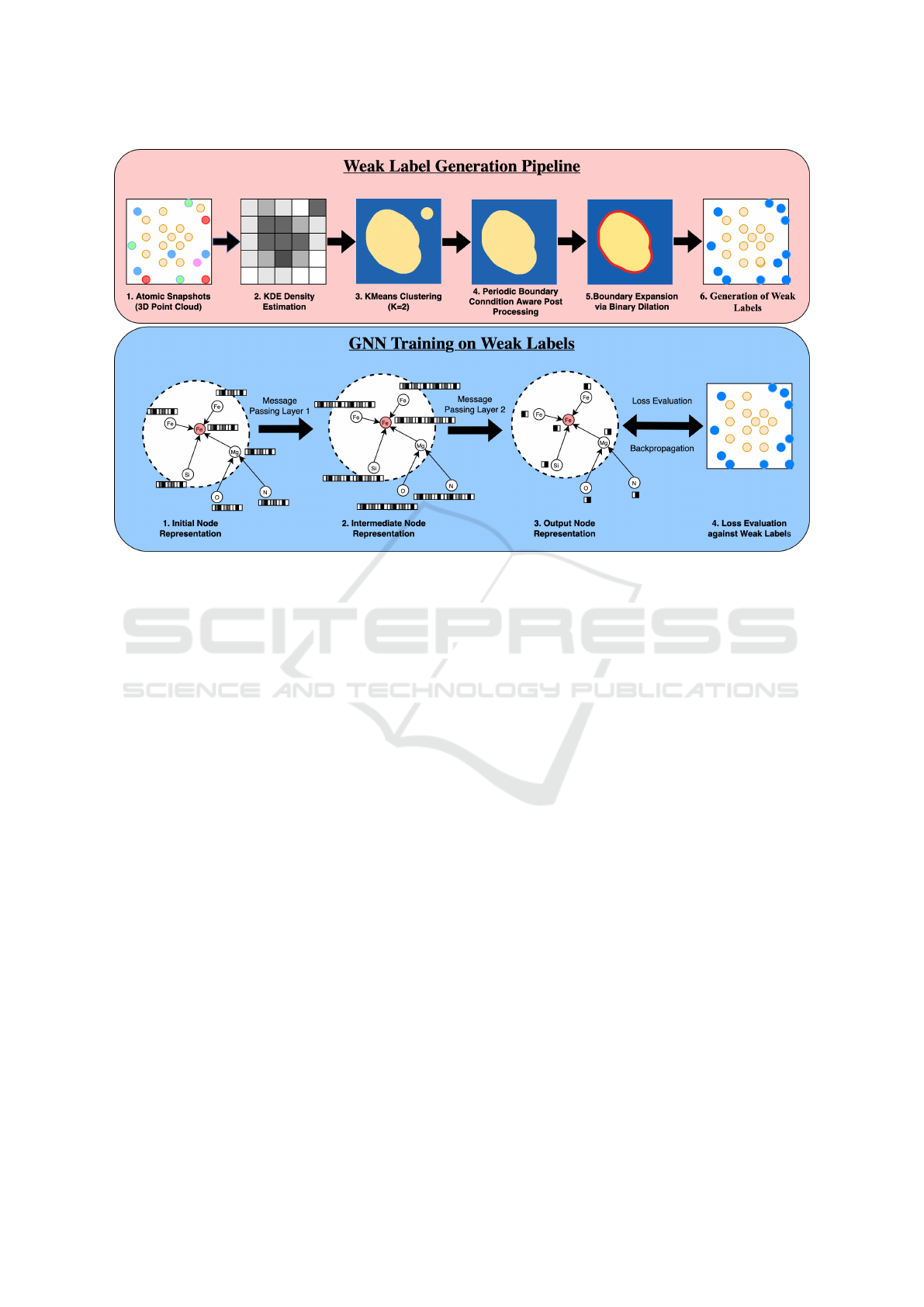
Figure 1: Schematic of the proposed phase segmentation approach. Top: Weak labels are generated via a pipeline that involves

KDE-based density estimation, clustering, Periodic Boundary Condition aware post-processing, and boundary (interface)

expansion using binary dilation. Bottom: A GNN is trained on these weak labels using node features based on atomic type

and local environment.

simulation snapshots for different boundary widths

and select the value that minimizes this variance, in-

dicating improved stability in phase classiﬁcation and

reduced ambiguity at the interface.

3.1.5 Label Assignment to Atoms

To generate per-atom labels, we map each atomic

position to its corresponding voxel in the clustered

density grid. The voxel’s pre-assigned phase la-

bel—either Fe-rich metal, Fe-poor silicate, or bound-

ary—is transferred to all atoms whose positions fall

within that voxel. This mapping ensures consistency

between the density-based voxel segmentation and

the atom-level labels required for model training. Be-

cause the voxel grid spans the entire simulation cell,

every atom is assigned a label based on its spatial lo-

cation relative to the phase-separated structure. This

process results in a fully labeled dataset of atoms,

where each atom inherits the phase identity of its local

environment as inferred from the KDE-based cluster-

ing and post-processing pipeline. These labels serve

as weak supervision targets for training our graph

neural network model.

3.2 GNN Training on Weak Labels

We formulate a semantic phase segmentation as a

node classiﬁcation task on atomic graphs, where su-

pervised learning is performed using weak labels de-

rived from our physics-informed pipeline. This ap-

proach tests whether a lightweight graph neural net-

work can replicate the accuracy of our computation-

ally intensive density-based method while achieving

superior scalability. To evaluate the generality of

our learning framework, we implement two different

GNN architectures—GCN and GAT—using identical

feature inputs and training protocols. This compara-

tive setup allows us to assess whether our weak super-

vision strategy is compatible with different message-

passing schemes.

3.2.1 Graph Representation and Node Features

Each atomic conﬁguration is represented as an undi-

rected graph G = (V, E), where each node v

∈ V cor-

responds to an atom, and an edge (i, j) ∈ E connects

atoms i and j if their spatial separation is less than a

predeﬁned cutoff distance r

. To preserve the phys-

ical continuity of the atomic environment, we apply

periodic boundary conditions (PBC) during neighbor

search using a wrapped distance metric.

Each node v

is associated with a feature vector

KDIR 2025 - 17th International Conference on Knowledge Discovery and Information Retrieval

306

∈ R

that encodes both chemical identity and local

structural information. The full node feature vector is

expressed as:

= concat



OneHot(type

), N

, µ

, σ

, f

, N



(1)

where N

denotes the number of Fe neighbors, µ

and σ

are the mean and variance of their distances,

is the fraction of Fe neighbors relative to total

neighbors, and N

is the count of Mg neighbors.

These features are chosen to reﬂect both the chem-

ical identity of the central atom and the local coordi-

nation environment, which are known to be predictive

of phase identity in metal-silicate systems. In par-

ticular, statistics over Fe neighbors help capture the

density and spatial distribution of metallic bonding,

while the inclusion of Mg neighbors aids in identify-

ing silicate-like environments. Neighbor counts for

Si and O were initially considered but later excluded

from the ﬁnal feature design, as they were found to be

redundant. Their inclusion had negligible impact on

the macro F1 score for GCN (0.878 vs. 0.873 without

them) and slightly reduced the performance of GAT

(0.809 vs. 0.819 without them), indicating that these

features do not contribute meaningfully to the phase

classiﬁcation task.

3.2.2 Message Passing and Prediction

Framework

GNNs operate by iteratively updating node represen-

tations through localized neighborhood aggregation.

For a given graph G = (V, E), with initial node fea-

tures h

(0)

= x

, each GNN layer reﬁnes node embed-

dings via:

(l+1)

= σ



AGG

(l)

n

(l)

| j ∈ N (i)

∪

(l)

o

(2)

where N (i) denotes the set of neighbors of node i,

σ is the ReLU activation function, and AGG

(l)

is the

layer-speciﬁc aggregation function.

Our model architecture consists of two such

message-passing layers, enabling nodes to incorpo-

rate information from both ﬁrst and second-order

neighborhoods. The output of the ﬁnal layer is a 2-

dimensional embedding used for binary classiﬁcation

(Fe-rich vs. Fe-poor). These logits are converted into

class probabilities using a softmax function:

= softmax(h

(L)

), (3)

where L is the total number of layers.

We implement and evaluate two GNN variants,

each employing a different aggregation strategy:

GraphConv: The GraphConv operator uses nor-

malized aggregation as follows:

(l+1)

= σ





∑

j∈N (i)∪{i}

|N (i)| |N ( j)|

(l)





(4)

GAT: Graph Attention Networks introduce learn-

able attention weights between neighbors:

(l+1)

= σ





∑

j∈N (i)

(l)

i j

(l)





, (5)

with attention coefﬁcients computed as:

(l)

i j

exp



⊤

(l)

∥ W

(l)

i

∑

k∈N (i)

exp



⊤

(l)

∥ W

(l)

i

(6)

where W

(l)

∈ R

′

×d

is a learnable weight matrix,

a ∈ R

′

is a learnable attention weight vector, ∥ de-

notes vector concatenation, and f is the LeakyReLU

activation function.

Training Objective. The network is trained using

the standard cross-entropy loss, deﬁned over the set

of weakly labeled atoms:

L = −

∑

i∈T

∑

c=1

log ˆy

, (7)

where T is the set of labeled atoms, y

∈ {0, 1} is

the one-hot encoded ground truth weak label, and ˆy

is the predicted class probability from Equation 3.

Training is performed using the Adam optimizer, with

both models trained under the same hyperparameter

settings.

4 EXPERIMENTS AND RESULTS

4.1 Weak Label Generation

We ﬁrst evaluate the effectiveness of our weak la-

beling pipeline on a small FeMgSiON system con-

taining 520 atoms in a cubic simulation supercell

of 17

A length. Each atom is assigned a phase

label—Fe-rich (metal), Fe-poor (silicate), or bound-

ary/interface—based on its spatial location within a

voxelized grid, where each voxel is classiﬁed into one

of the three regions. Atoms inherit the phase label of

the voxel they fall into.

Weakly Supervised Graph Neural Networks for Scalable 3D Phase Segmentation in Molecular Dynamics Simulations

307

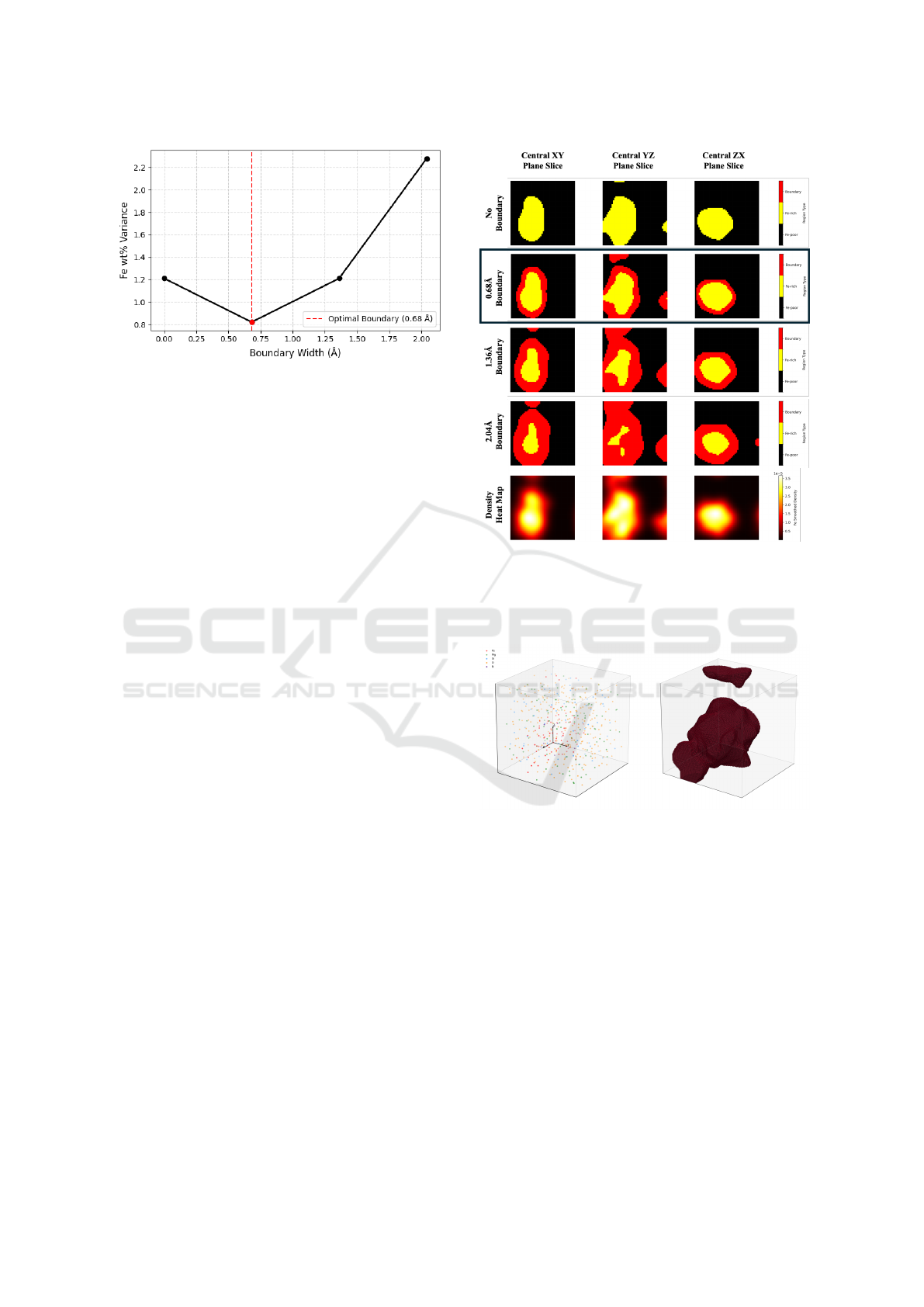
Figure 2: Variance of Fe weight percent in the Fe-rich re-

gion across 1000 snapshots from the 3000 K simulation,

plotted as a function of boundary width.

A critical hyperparameter in this labeling process

is the boundary width, which determines how many

voxels are designated as interfacial (boundary) rather

than purely Fe-rich or Fe-poor. To determine an ap-

propriate value, we evaluate the variance of Fe weight

percent in the Fe-rich region across 1000 simulation

snapshots, under different boundary thicknesses. As

shown in Figure 2, a boundary width of 0.68

A re-

sults in the lowest variance, indicating greater stabil-

ity in the phase classiﬁcation and reduced ambiguity

at the interface. While this analysis was conducted at

3000 K, we found that the same boundary width also

yielded the lowest variance for simulations at 4000 K.

We visualize how different boundary widths affect

segmentation outcomes in Figure 3, which shows cen-

tral XY, YZ, and XZ slices of a representative snap-

shot. Without a boundary region, the segmentation is

overly sharp and fails to capture the transitional na-

ture of the interface. Introducing a 0.68

A boundary

produces smoother, more physically realistic segmen-

tation. Larger boundaries (1.36

A, 2.04

A) begin to

erode phase interiors, reducing ﬁdelity.

To assess the spatial coherence and physical plau-

sibility of the assigned labels, we visualize the Fe-rich

region from a reference snapshot. As shown in Fig-

ure 4, the segmented metallic domain forms a large,

continuous structure consistent with physical expec-

tations for phase-separated systems. Although the vi-

sualization shows two disconnected volumes, they be-

long to a single contiguous phase, split only by peri-

odic boundaries. Our labeling method accounts for

this, correctly identifying such regions as topologi-

cally connected. This conﬁrms that the chosen bound-

ary width and labeling approach preserve spatial con-

tinuity and yield stable, physically meaningful phase

assignments suitable for training downstream models.

Figure 3: Phase segmentation slices across three planes

(XY, YZ, XZ) for different boundary sizes in the 3000 K

simulation. Rows show no boundary, 0.68

A, 1.36

A, and

2.04

A, respectively. The 0.68

A boundary best preserves

phase boundaries without distorting region interiors.

Figure 4: 3D visualization of phase segmentation. Left:

Atom positions with species color-coded. Right: Seg-

mented Fe-rich region rendered as a connected volume. The

split appearance is due to periodic boundaries; the region is

physically continuous.

4.2 Phase Segmentation with

Graph-Based Models

We conducted experiments on two distinct FeMg-

SiON systems—one at 29 GPa and 3000 K, and an-

other at 35 GPa and 4000 K. For each condition, sim-

ulations were performed at two different scales. Each

system was simulated at two scales: a small system

(520 atoms) used for training, and a large system

(33,280 atoms) used for inference and validation. The

small and large systems were constructed with identi-

KDIR 2025 - 17th International Conference on Knowledge Discovery and Information Retrieval

308

cal elemental ratios, differing only in spatial scale and

total number of atoms.

For each temperature-pressure condition, we

trained GNNs independently on the small system.

Speciﬁcally, we used two architectures—GAT and

GCN—and evaluated their performance on the corre-

sponding large system. We benchmarked their out-

puts against labels generated by our unsupervised

pipeline, which serves as a high-ﬁdelity—but com-

putationally expensive reference.

4.3 Results and Analysis

To evaluate classiﬁcation performance, we tested two

GNN architectures—GAT and GCN—on large-scale

FeMgSiON systems at two thermodynamic states.

Both models were trained on small systems using

weak labels derived from our unsupervised segmen-

tation pipeline and evaluated on larger systems using

the following metrics:

• Elemental weight percent (wt%) in predicted Fe-

rich (metal) and Fe-poor (silicate) regions, aver-

aged over 100 snapshots,

• Classiﬁcation accuracy and F1 scores (micro,

macro, and per-class),

• ROC curves and confusion matrices for model

comparison.

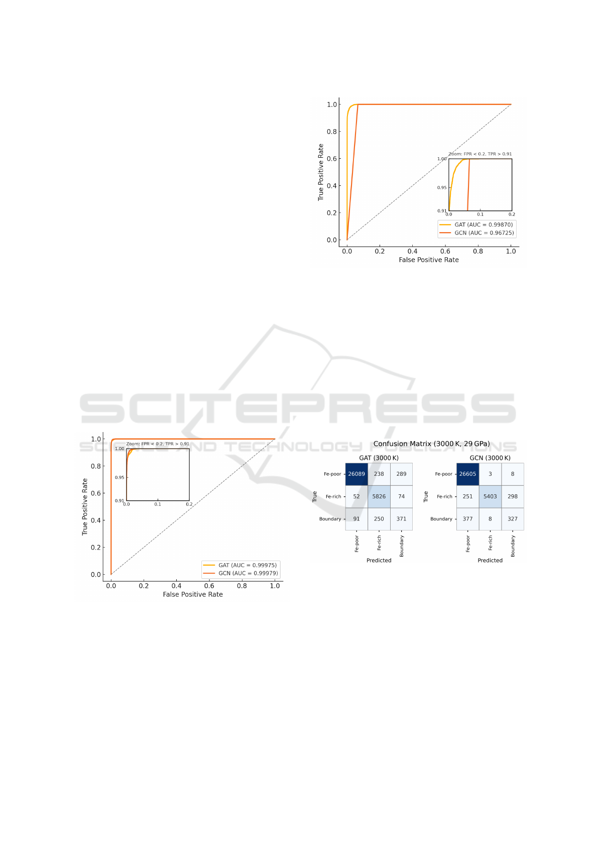
Figure 5: ROC curve comparing the classiﬁcation perfor-

mance of GAT and GCN models on the reference snapshot

of the 3000 K, 29 GPa simulation. The inset highlights the

region with low false positive rates and high true positive

rates.

At 3000 K, where thermal agitation is minimal

and phase boundaries are sharply deﬁned, both GAT

and GCN generalize well from the small training sys-

tem to the large-scale target. The confusion matri-

ces (Figure 7) show strong diagonal dominance, and

Figure 6: ROC curve comparing the classiﬁcation perfor-

mance of GAT and GCN models on the reference snapshot

of the 4000 K, 35 GPa simulation. The inset highlights the

region with low false positive rates and high true positive

rates, showing ﬁner differences in model sensitivity.

the ROC curves (Figure 5) conﬁrm near-perfect sep-

arability, with area under the curve (AUC) exceeding

0.999 for both models. These high AUC values reﬂect

threshold-agnostic discriminative performance, indi-

cating that both GNNs reliably distinguish Fe-rich,

Fe-poor, and boundary atoms across a range of thresh-

olds. The macro F1 scores also exceed 0.85, under-

scoring consistent performance across all classes (Ta-

ble 1).

Figure 7: Confusion matrices for Fe-rich, Fe-poor, and

boundary classiﬁcation at 3000 K and 29 GPa using GAT

and GCN. Shown for the reference snapshot of our large-

scale simulation (33,280 atoms), predictions are bench-

marked against labels obtained from the high-ﬁdelity un-

supervised segmentation pipeline.

At 4000 K, increased thermal mixing introduces

ambiguity in phase boundaries, making segmenta-

tion more difﬁcult. GCN’s performance degrades sig-

niﬁcantly, particularly in its ability to detect bound-

ary regions, as reﬂected in a low boundary F1 score

(0.06). Its AUC also drops to 0.967, indicating re-

duced conﬁdence in its ranking. While GCN cor-

rectly classiﬁes nearly all Fe-rich (Metal) phase atoms

Weakly Supervised Graph Neural Networks for Scalable 3D Phase Segmentation in Molecular Dynamics Simulations

309

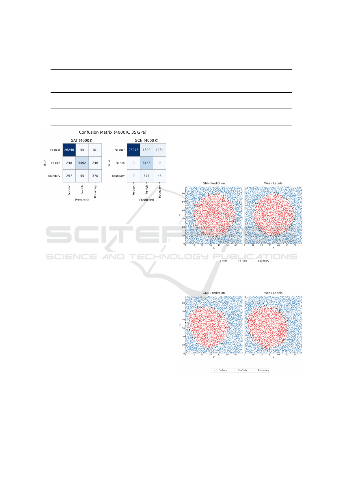
Table 1: Classiﬁcation performance of GNN models across systems. Reported values include accuracy, class-wise F1 scores,

macro F1, and micro F1 scores.

System Model Accuracy

(Fe-Poor/

Silicate)

(Fe-Rich/

Metal)

(Boundary)

Macro

Micro

3000 K, 29.1 GPa

GAT 0.979 0.986 0.964 0.506 0.819 0.979

GCN 0.986 0.995 0.945 0.678 0.873 0.986

4000 K, 35 GPa

GAT 0.975 0.986 0.929 0.515 0.810 0.975

GCN 0.899 0.926 0.866 0.061 0.618 0.899

Figure 8: Confusion matrices for Fe-rich, Fe-poor, and

boundary classiﬁcation at 4000 K and 35 GPa using GAT

and GCN. Shown for the reference snapshot of our large-

scale simulation (33,280 atoms), predictions are bench-

marked against labels obtained from the high-ﬁdelity un-

supervised segmentation pipeline.

at 4000 K (see Figure 8), it fails to resolve transi-

tional regions, misclassifying most boundary atoms

as Fe-rich—highlighting its limited capacity to cap-

ture compositional shifts in disordered systems. In

contrast, GAT maintains strong performance, with

an AUC above 0.998 and a macro F1 of 0.81. We

attribute this robustness to its attention mechanism,

which adaptively weighs contributions from neigh-

boring atoms and remains effective even under high-

temperature, disordered conditions.

Table 2 summarizes the average elemental com-

positions (wt%) predicted for Fe-rich/Metal and Fe-

poor/Silicate phases under both 3000 K/29 GPa and

4000 K/35 GPa conditions. At 3000 K, both GNN

models closely match the unsupervised baseline, in-

dicating accurate phase segmentation under low mix-

ing. At 4000 K, GCN predictions deviate more no-

ticeably from the unsupervised results—particularly

in Fe and Mg content—while GAT continues to pro-

duce more consistent estimates. These trends high-

light the improved reliability of GAT in capturing

phase behavior under more challenging thermody-

namic conditions.

Figures 9 and 10 show the XY projections of

atoms whose Z-bins lie between 20 and 30 from the

reference test snapshots of the large-scale systems at

29 GPa and 3000 K, and 35 GPa and 4000 K, respec-

tively. In both cases, this representative slice is ex-

tracted from a 50×50×50 spatial grid. These visual-

izations compare the GNN predictions against weak

labels to qualitatively assess the model’s ability to re-

cover physically meaningful phase separation into Fe-

rich, Fe-poor, and boundary regions.

Figure 9: XY projection of atoms from the central Z slice

of our reference snapshot in the 3000 K, 29 GPa system,

comparing GNN predictions with weak labels.

Figure 10: XY projection of atoms from the central Z slice

of our reference snapshot in the 4000 K, 35 GPa system,

comparing GNN predictions with weak labels.

Beyond segmentation accuracy, a key advantage

of our graph-based approach is its speed at inference

time. In particular, we compare the inference time of

KDIR 2025 - 17th International Conference on Knowledge Discovery and Information Retrieval

310

Table 2: Average elemental composition (wt%) in Fe-rich (Metal) and Fe-poor (Silicate) regions for both sys-

tems—3000 K/29 GPa and 4000 K/35 GPa—as predicted by GAT, GCN, and the unsupervised baseline. Values are averaged

over 100 test snapshots; standard error is reported.

T–P Phase Method Fe (wt %) Mg (wt %) Si (wt %) O (wt %) N (wt %)

3000 K, 29 GPa

Fe-rich

(Metal)

GAT 93.22 ± 0.18 0.06 ± 0.18 1.61 ± 0.10 1.83 ± 0.07 3.20 ± 0.00

GCN 94.64 ± 0.20 0.00 ± 0.00 1.57 ± 0.12 0.72 ± 0.08 3.05 ± 0.02

Unsupervised 93.81 ± 0.21 0.10 ± 0.01 1.67 ± 0.12 1.27 ± 0.09 3.15 ± 0.01

Fe-poor

(Silicate)

GAT 1.23 ± 0.07 29.45 ± 0.02 23.06 ± 0.05 46.13 ± 0.03 0.11 ± 0.00

GCN 5.06 ± 0.12 28.04 ± 0.02 22.06 ± 0.06 44.56 ± 0.05 0.28 ± 0.00

Unsupervised 3.77 ± 0.08 28.53 ± 0.02 22.39 ± 0.05 45.10 ± 0.03 0.19 ± 0.00

4000 K, 35 GPa

Fe-rich

(Metal)

GAT 90.59 ± 0.03 0.10 ± 0.01 2.99 ± 0.03 3.06 ± 0.04 3.25 ± 0.01

GCN 80.27 ± 0.25 3.41 ± 0.10 5.11 ± 0.05 8.41 ± 0.14 2.87 ± 0.01

Unsupervised 89.54 ± 0.01 0.37 ± 0.01 3.35 ± 0.03 3.52 ± 0.02 3.22 ± 0.02

Fe-poor

(Silicate)

GAT 3.47 ± 0.04 29.28 ± 0.01 22.07 ± 0.01 45.03 ± 0.02 0.14 ± 0.01

GCN 2.17 ± 0.04 29.82 ± 0.04 22.30 ± 0.06 45.68 ± 0.06 0.08 ± 0.00

Unsupervised 5.79 ± 0.05 28.49 ± 0.02 21.47 ± 0.02 44.07 ± 0.01 0.19 ± 0.01

our trained GNNs against the original unsupervised

pipeline used for generating weak labels. All infer-

ences were conducted on the 33,280-atom large-scale

system using non-parallelized implementations. To

ensure fair comparison, all methods were executed on

identical hardware with the same processor conﬁgu-

ration.

Table 3: Inference time and scaling behavior of different

segmentation methods, reported over 100 test snapshots

from the 33,280-atom large-scale system. Values reﬂect the

mean and standard error.

Method Time (s) Scaling

GNN (GAT) 3.61 ± 0.12 ∼ O(N)

GNN (GCN) 3.12 ± 0.14 ∼ O(N)

Unsupervised 210.0 ± 2.2 O(N · M)

(KDE + Clustering)

GNN inference comprises two steps: graph con-

struction and forward propagation. Graph construc-

tion uses a ﬁxed-radius neighbor search with spatial

indexing (e.g., cKDTree), scaling approximately lin-

early with system size. The forward pass involves a

constant number of message-passing layers and also

scales linearly with the number of atoms. In contrast,

the unsupervised pipeline involves kernel density es-

timation (KDE) over a 3D voxel grid, followed by

clustering and morphological post-processing. KDE

requires each atom to contribute to many voxels, re-

sulting in O(N · M) complexity, where N is the num-

ber of atoms and M the number of voxels—making

it a computational bottleneck for large-scale simula-

tions.

As shown in Table 3, our GNN models reduce

inference time from over 200 seconds to just over

3 seconds for the 33,280-atom system—achieving a

speedup of over two orders of magnitude. This high-

lights their efﬁciency over the original unsupervised

pipeline and suitability for large-scale applications.

5 CONCLUSIONS

We introduced a hybrid learning approach for scal-

able and accurate phase segmentation in large-scale

molecular dynamics simulations by combining a

structure-aware unsupervised pipeline with a weakly-

supervised GNNs. This approach enables model

training even in the absence of labeled data by lever-

aging structural heuristics to generate weak supervi-

sion. The GNNs are trained on small systems but gen-

eralize effectively to much larger conﬁgurations with-

out sacriﬁcing accuracy, demonstrating robust perfor-

mance across varying system sizes. Among the ar-

chitectures evaluated, GATs in particular showed con-

sistent performance across systems with different de-

grees of disorder, effectively capturing boundary re-

gions. As parametric models, they offer signiﬁcant

speedups during inference by eliminating the need

for repeated unsupervised computations, with runtime

beneﬁts that grow with system size. While demon-

strated on FeMgSiON systems, the strategy is broadly

applicable to other multi-phase materials where high-

quality labels are unavailable but structural cues ex-

ist. These results underscore a broader opportunity

in using machine learning to accelerate and scale sci-

entiﬁc analyses in domains where conventional la-

beling is impractical. A promising direction for

future work is the integration of uncertainty-aware

active learning, where the model identiﬁes regions

of low conﬁdence—particularly near phase bound-

aries—and selectively queries for additional weak su-

pervision. Techniques such as Monte Carlo Dropout

Weakly Supervised Graph Neural Networks for Scalable 3D Phase Segmentation in Molecular Dynamics Simulations

311

or Bayesian GNNs could be employed to estimate

uncertainty, allowing the model to prioritize ambigu-

ous regions and further improve segmentation quality

while minimizing labeling overhead.

ACKNOWLEDGEMENTS

This work was supported by NASA (Grant No.

80NSSC21K0377) and the National Science Founda-

tion (EAR 1463807). Computational resources were

provided by the High Performance Computing facil-

ity at Louisiana State University. Additional support

was received through the Summer Opportunities Fel-

lowship, awarded by Shell Oil Company.

REFERENCES

Chazelle, B. (1993). An optimal convex hull algorithm in

any ﬁxed dimension. Discrete & Computational Ge-

ometry, 10(4):377–409.

Chen, L.-C., Papandreou, G., Kokkinos, I., Murphy, K.,

and Yuille, A. L. (2017). Rethinking atrous convo-

lution for semantic image segmentation. IEEE Trans-

actions on Pattern Analysis and Machine Intelligence

(TPAMI), 39(12):2341–2355.

Edelsbrunner, H. and M

ucke, E. P. (1994). Three-

dimensional alpha shapes. ACM Transactions on

Graphics (TOG), 13(1):43–72.

Fukuya, T. and Shibuta, Y. (2020). Machine learning ap-

proach to automated analysis of atomic conﬁguration

of molecular dynamics simulation. Computational

Materials Science, 184:109880.

Hamilton, W. L., Ying, R., and Leskovec, J. (2017). In-

ductive representation learning on large graphs. In

Advances in Neural Information Processing Systems

(NeurIPS).

Honeycutt, J. and Andersen, H. (1987). Molecular dynam-

ics study of melting and freezing of small lennard-

jones clusters. The Journal of Physical Chemistry,

91(19):4950–4963.

Jadrich, R. B., Lindquist, B. A., and Truskett, T. M. (2018).

Unsupervised machine learning for detection of phase

transitions. Physical Review E, 97:023301.

Kipf, T. N. and Welling, M. (2017). Semi-supervised clas-

siﬁcation with graph convolutional networks. In In-

ternational Conference on Learning Representations

(ICLR).

Long, J., Shelhamer, E., and Darrell, T. (2015). Fully con-

volutional networks for semantic segmentation. In

Proceedings of the IEEE Conference on Computer Vi-

sion and Pattern Recognition (CVPR), pages 3431–

3440.

Lopez, C. A., Vesselinov, V. V., Gnanakaran, S., and

Alexandrov, B. S. (2019). Unsupervised machine

learning for analysis of coexisting lipid phases and

domain growth in biological membranes. bioRxiv,

527630(v2). Preprint, version 2.

MacQueen, J. (1967). Some methods for classiﬁcation and

analysis of multivariate observations. In Proceed-

ings of the Fifth Berkeley Symposium on Mathematical

Statistics and Probability, Volume 1: Statistics, pages

281–297. University of California Press.

McDonough, W. F. and Sun, S.-S. (1995). The composition

of the Earth. Chemical Geology, 120(3–4):223–253.

Qi, C. R., Su, H., Mo, K., and Guibas, L. J. (2017). Pointnet:

Deep learning on point sets for 3d classiﬁcation and

segmentation. In Proceedings of the IEEE Conference

on Computer Vision and Pattern Recognition (CVPR),

pages 652–660.

Ronneberger, O., Fischer, P., and Brox, T. (2015). U-net:

Convolutional networks for biomedical image seg-

mentation. Medical Image Computing and Computer-

Assisted Intervention (MICCAI), 9351:234–241.

Scarselli, F., Gori, M., Tsoi, A. C., Hagenbuchner, M.,

and Monfardini, G. (2009). The graph neural net-

work model. IEEE Transactions on Neural Networks,

20(1):61–80.

Serra, J. (1982). Image analysis and mathematical morphol-

ogy. Academic Press.

Shakya, A., Ghosh, D. B., Jackson, C., Morra, G., and

Karki, B. B. (2024). Insights into core–mantle differ-

entiation from bulk earth melt simulations. Scientiﬁc

Reports, 14(1):18739.

Silverman, B. W. (1986). Density Estimation for Statistics

and Data Analysis. Chapman and Hall/CRC.

Stukowski, A. (2012). Structure identiﬁcation methods for

atomistic simulations of crystalline materials. Mod-

elling and Simulation in Materials Science and Engi-

neering, 20(4):045021.

Veli

ckovi

c, P., Cucurull, G., Casanova, A., Romero, A., Li

P., and Bengio, Y. (2018). Graph attention networks.

In International Conference on Learning Representa-

tions (ICLR).

Virtanen, P., Gommers, R., Oliphant, T. E., and ... (2020).

SciPy 1.0: Fundamental algorithms for scientiﬁc com-

puting in python. Nature Methods, 17:261–272.

Zhang, Y. and Guo, G. (2009). Partitioning of si and o

between liquid iron and silicate melt: A two-phase

ab initio molecular dynamics study. Geophysical Re-

search Letters, 36(18):L18305.

KDIR 2025 - 17th International Conference on Knowledge Discovery and Information Retrieval

312