Reinforcement Learning for Model-Free Control of a Cooling Network

with Uncertain Future Demands

Jeroen Willems

, Denis Steckelmacher

, Wouter Scholte

, Bruno Depraetere

, Edward Kikken

Abdellatif Bey-Temsamani

and Ann Nowé

Flanders Make, Lommel, Belgium

Vrije Universiteit Brussel, Belgium

ﬁ ﬂ ﬁ

Keywords:

Predictive Control, Reinforcement Learning, Thermal Systems Control.

Abstract:

Optimal control of complex systems often requires access to a high-ﬁdelity model, and information about the

(future) external stimuli applied to the system (load, demand, ...). An example of such a system is a cooling

network, in which one or more chillers provide cooled liquid to a set of users with a variable demand. In this

paper, we propose a Reinforcement Learning (RL) method for such a system with 3 chillers. It does not assume

any model, and does not observe the future cooling demand, nor approximations of it. Still, we show that, after

a training phase in a simulator, the learned controller achieves a performance better than classical rule-based

controllers, and similar to a model predictive controller that does rely on a model and demand predictions. We

show that the RL algorithm has learned implicitly how to anticipate, without requiring explicit predictions. This

demonstrates that RL can allow to produce high-quality controllers in challenging industrial contexts.

1 INTRODUCTION

Today, reducing the energy consumption of industrial

systems is a key challenge. Energy reduction can be

achieved by designing more efﬁcient systems, but of-

ten improvements can be made by improving the way

they are controlled. Academically optimization-based

model-based controllers are often proposed when more

advanced control is required. While these are effec-

tive, they introduce signiﬁcant complexity due to the

need for accurate models and powerful optimizers that

run during system operation. Therefore, in industry

the adoption is still rather limited. In this work, we

explore reinforcement learning (RL) as a simpler, data-

driven alternative that requires neither. We benchmark

its performance against both model-based and simpler

rule-based control (still widely used in industry) by

evaluating them on a thermal system comprised of

three interconnected chillers.

For the model-based controller in this paper, we

consider the optimal control of a dynamic system.

As time passes, with time denoted by

, the system

changes state. The state of the system at some time

is denoted

(

). Some control signal applied to the sys-

tem at time

is denoted

(

), and the resulting change

of state is denoted

˙x

(

) =

f [x(t),u(t),t]

. The function

deﬁnes how the system reacts to the control signal.

It also depends on

, which allows the function to addi-

tionally depend on non-controlled information, such

as the weather (that we cannot inﬂuence), some usage

of the system by clients, etc.

The objective of optimal control is to produce con-

trol signals

(

) such that, over some time period, a

cost function dependent on the system states is mini-

mized. Instances of optimal control include moving

towards and tracking a setpoint, tracking some (mov-

ing) reference signal, or performing a task while mini-

mizing energy consumption. Methods that attempt to

achieve optimal control range from simple to very com-

plicated, starting from proportional-integral-derivative

controllers (Borase et al., 2021), over optimal feedback

design methods like linear quadratic regularors and H-

inﬁnity (Glover, 2021), to function optimization - such

as gradient methods (Mehra and Davis, 1972), genetic

algorithms (Michalewicz et al., 1992), ant-colony op-

timization (López-Ibáñez et al., 2008), iterated local

search methods (Lourenço et al., 2019) - and especially

optimal control, with its continuous and discrete time,

direct and indirect, and many more variants (Lewis

et al., 2012), and its implementation that adds robust-

ness through feedback called model-predictive control

or MPC (Camacho and Alba, 2013). Conceptually,

MPC observes the current state of the system, then

uses a computational model of it to predict various

Willems, J., Steckelmacher, D., Scholte, W., Depraetere, B., Kikken, E., Bey-Temsamani, A. and Nowé, A.

Reinforcement Learning for Model-Free Control of a Cooling Network with Uncertain Future Demands.

DOI: 10.5220/0013708300003982

Paper published under CC license (CC BY-NC-ND 4.0)

In Proceedings of the 22nd International Conference on Informatics in Control, Automation and Robotics (ICINCO 2025) - Volume 1, pages 59-70

ISBN: 978-989-758-770-2; ISSN: 2184-2809

possible outcomes, so the best-possible control signal

can be chosen by a numerical optimization problem.

Apart from the PID approach, all these methods

share a common trait: they are model-based. They

assume that

f [x(t),u(t),t]

is available, in a represen-

tation that can be used to design a controller or to

compute control signals. This means that the system

must be modelled, along with any function of

used

. When relevant, they further include predictions

on expected future events as well, using the model to

predict how to best anticipate on those events.

However, in the real world, models are never per-

fect, and future demands are not always known per-

fectly. Methods exist to estimate models, or future de-

mands, for instance with Kalman ﬁlters (Meinhold and

Singpurwalla, 1983) or machine learning approaches

such as time-series prediction (Frank et al., 2001).

These methods are unfortunately approximate, and

prevent optimal control from being achieved.

We propose to instead use another method of pro-

ducing control signals: Reinforcement Learning (RL)

is a family of machine learning (ML) algorithms that

allows to learn a controller from experience. The im-

portant property of RL, that we explain extensively in

Section 2, is that it is model-free. The RL agent, that

learns the controller, makes no assumption about the

system being controlled, and does not expect to have

access to its state update function

or to the future

demands

RL has already been applied to numerous cases

in research settings, like video games and (simulated)

robotic tasks. Real-life application to industrial appli-

cations is more rare, though there are examples that go

in that direction, like optimizing combustion in coal-

ﬁred power plants (Zhan et al., 2022), cooling for data

centers (Luo et al., 2022), application to Domestic Hot

Water (DHW) systems (De Somer et al., 2017) and

systems of compressors (Chen et al., 2024).

In this paper, we will tackle a cooling problem,

somewhat similar to (Luo et al., 2022), with both

continuous (power levels) as well as discrete (on/off)

control actions, and a non-instantaneous objective to

minimize energy with penalties for frequent on/off

switches. We will use existing RL techniques, and

compare it to other approaches, since like mentioned

above, such a problem would typically be tackled with

MPC-like controllers that use a model, as well as a

prediction of the upcoming demand.

Our contributions are as follows:

•

We explain how to set up and formulate the RL

problem for this application, relying on existing

Some RL methods are called model-based because the

RL agent learns an approximate model of

, but the true

still not observed by the agent.

state-of-the-art RL algorithms for solving it.

•

For this application, we present evaluations and

comparisons of a rule-based controller or RBC

(which is the industrial standard), an MPC, and

an RL controller, showing that both MPC and RL

outperform the RBC.

•

We study the impact of imprecise or limited pre-

view information on upcoming demand for the

MPC, and compare it to the RL to show that the

RL learns to anticipate even without being given

explicit preview information.

2 BACKGROUND

2.1 Reinforcement Learning

RL is a machine learning approach that allows to learn

a closed-loop controller from experience with the con-

trolled system. In most of the literature, RL considers

a discrete-time Markov Decision Process (MDP) de-

ﬁned by the tuple



S, A, R, T, µ

, γ



, with

the space

of states,

the space of actions,

S × A → R

the

reward function that maps a state-action pair to a scalar

reward,

S × A × S →

1] the transition function

that describes the probability that an action in a state

leads to some next state,

the initial state distribution,

and γ < 1 the discount factor.

In physical applications, the state-space is usually

a subspace of

, vectors of

real numbers. The

action space can either be discrete, with the action

being one of some ﬁnite set of possible actions, or

continuous, with the action space a subspace of R

RL considers multi-step decision making. Time is

divided in discrete time-steps, and several time-steps

form an episode. When an episode ends, the MDP

is reset to an initial state drawn from

, and a new

episode starts. The objective of a RL agent is to learn

an optimal (possibly stochastic) policy

(

a|s

) such

that, when following that policy, the expected sum of

discounted rewards

∑

(

, a

∼ π

(

)) per episode

is as high as possible.

For RL the learning agent does not have to have

access to the reward or transition functions, it can get

by with just evaluations, by e.g. interacting physically

with a non-modelled plant. As such, the reward func-

tion can be implemented in any way suited for the task,

and the transition function does not even have to exist

in a computer format.

ICINCO 2025 - 22nd International Conference on Informatics in Control, Automation and Robotics

2.2 POMDPs

Partially-Observable Markov Decision Processes

(Monahan, 1982) (POMDP) consider the setting in

which the agent does not have access to the state of

the process being controlled, but only a (partial) ob-

servation. A POMDP extends the MDP with the

observation space, and the Ω :

S → O

observation func-

tion. The reward function still depends on the state:

the agent is now rewarded according to information it

may not observe.

POMDPs are extremely challenging to tackle, as

the framework does not impose any lower bound on

what the agent observes. No general solution is there-

fore available. However, methods that try to infer what

the hidden state is (Roy and Gordon, 2002), methods

in which the agent reasons about past observations

using recurrent neural networks (Bakker, 2001), and

methods that give a history of past observations as in-

put to the agent (Mnih et al., 2015; Shang et al., 2021)

currently perform the best.

We observe that POMDPs still assume that there

is a hidden state, from which the reward function and

next state are computed. This is not the case in the

setup we introduce later, in which the future demand

of cooling is not known to the agent, and not part of

the state. It is an external signal that, in the real world,

comes from the users and is not modeled. We still

observe that the ’history of past observations’ approach

to POMDPs helps the agent in our setup, even if our

setup is even more complicated than a POMDP.

2.3

Reinforcement Learning Algorithms

RL algorithms allow an agent to learn a (near-)optimal

policy in a Markov Decision Process. In this article,

we focus on on-line model-free RL algorithms: they in-

teract with the environment (or a simulation of it), and

learn from these interactions without using a model of

the environment, or trying to learn one.

Such RL algorithms are divided in three main fam-

ilies: value-based, that learn how good an action is

in a given state, policy-based, that directly learn how

much an action should be performed in a state, and

actor-critic algorithms, that learn both a value function

and a policy.

The best-known value-based algorithms are of the

family of Q-Learning (Watkins and Dayan, 1992),

with modern implementations being DQN (Mnih et al.,

2015) and its extensions, such as Prioritized DQN,

The simulator itself may be considered a model of the

environment, but can be approximate, does not need to be

differentiable, and is not given to the agent.

Dueling DQN or Quantile DQN, discussed and re-

viewed by (Hessel et al., 2018). The main proper-

ties of value-based algorithms is that they are sample-

efﬁcient, they learn with few interactions with the en-

vironment, but are in the vast majority of cases only

compatible with discrete actions. Despite some con-

tributions in that direction (Van Hasselt and Wiering,

2007; Asadi et al., 2021), value-based algorithms do

not scale well to, or do not match policy-based meth-

ods in high-dimensional high-complexity continuous-

action industrial tasks.

Policy-based algorithms historically started with

REINFORCE (Williams, 1992), followed by Policy

Gradient (Sutton et al., 1999), still the basis of al-

most every current policy-based or actor-critic algo-

rithm. Most modern policy-based algorithms are actu-

ally actor-critic, because they learn some sort of value

function (or Q-Values) in parallel with training the

actor with a variation of Policy Gradient. Examples

include Trust Region Policy Optimization (Schulman

et al., 2015), Proximal Policy Optimization (Schulman

et al., 2017) and the Soft Actor-Critic (Haarnoja et al.,

2018), the current state of the art. Deterministic Policy

Gradient (Silver et al., 2014) (DPG) is worth mention-

ing because it learns a deterministic policy (given a

state, it produces an action), as opposed to the other

approaches that are stochastic (given a state, they pro-

duce a probability distribution, usually the mean and

standard deviation of a Gaussian). A modern variant

of deep DPG (DDPG) is TD3 (Fujimoto et al., 2018),

that combines DDPG with advanced algorithms for

training the critic.

The main advantage of policy-based and actor-

critic algorithms is that they are compatible with con-

tinuous actions. In this article, we therefore focus

on them, and use Proximal Policy Optimization in

particular, after we observed that it outperforms the

Soft Actor-Critic in our setting. A plausible expla-

nation for this surprising result (SAC is more recent

than PPO) is that SAC relies heavily on a state-action

critic, itself built on the mathematical assumptions of

a Markov Decision Process. Because our task is a

Partially-Observable Markov Decision Process, the

PPO algorithm, that makes less assumptions, is able

to learn more efﬁciently.

3 COOLING NETWORK SETUP

The particular use-case we consider in this paper is a

scaled down version of an industrial cooling network.

We will study a simulation model of the experimental

setup shown in Figure 1. To allow for easier testing

on this model and this setup, we consider a scaled

Reinforcement Learning for Model-Free Control of a Cooling Network with Uncertain Future Demands

cooling task: we perform a shorter cycle (5 or 10 min-

utes cycles vs. typical 24 or 48 hours cycles), and

we have scaled the losses so that typical trade-offs

as found in industrial cooling scenarios are present.

These rescaled losses ensure the controller faces the

typical industrial trade-off when deciding when and

how much to use the chillers: alternating between

on/off too often causes start/stop losses and wears out

the units, while keeping them on for longer durations

and building up a thermal buffer by cooling too much

will result in extra heat transfer losses to the environ-

ment.

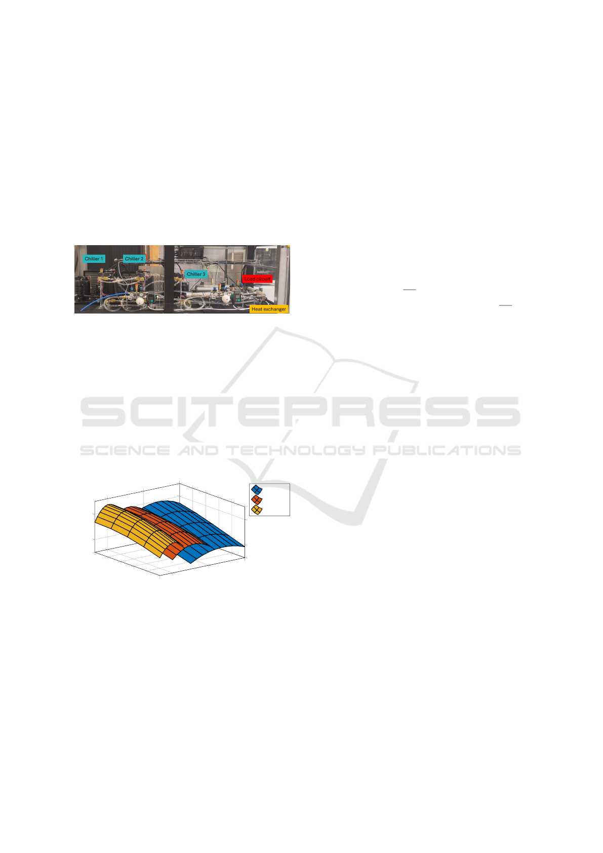
Figure 1: Experimental setup with 3 chillers and a load.

The considered system consists of:

•

A cooling circuit with three chillers, which con-

vert input electrical power

input

in to cool-

ing power

cool

, with a given coefﬁcient of

performance (CoP), such that

cool

(

T, P

input

) =

CoP

(

T, P

input

)

input

, see Figure 2. The chillers

have varying (electrical) power ranges: 300W-

600W, 200W-400W, 130W-260W. When running,

they cannot operate between 0W and the respective

lower bounds, but alternatively, the chillers can be

off (0W).

200

400

600

input

[W]

Temperature [

◦

CoP

Chiller 1

Chiller 2

Chiller 3

Figure 2: Operating region and CoP of the chillers.

•

The load circuit, containing 1.5L water. The rel-

atively small inertia of this load circuit is chosen

so testing can be sped up (control results are seen

quicker), but makes the system more challenging

to control. The load circuit is heated by a pro-

grammable heating element according to a given

power proﬁle

load

detailed later. This circuit aims

to mimic industrial cooling demands.

•

A heat exchanger and a set of pumps. On the cold

side a pump is there to ensure cold liquid ﬂows

from the chillers to the heat exchanger, and slightly

warmer liquid ﬂows back to them. On the hot side

another pump is present to ensure ﬂow from the

load circuit to the heat exchanger and back.

The system is modelled in a simpliﬁed form using a

single temperature

, assumed equal across the system.

We thus do not have separate states for cold and hot

sides, but simply assume the chillers as well as the

heater directly impact

. We also use

as the input

for our CoP’s. Given this, the dynamics of

can be

written as an ordinary differential equation (ODE):

T = C(−P

cool, total

+ P

load

− P

loss

(T )), (1)

where

cool, total

∑

i=3

i=1

cool

(

T, P

input

) with

the re-

spective chiller.

denotes the capacity, with

= 1

5 kg the mass of water and

= 4186

kgK

the

speciﬁc heat capacity. Second,

load

denotes the heat

injected on the load side. Last, the power loss in the

system is modelled using a lookup table dependent

, with more power lost to the environment as

becomes lower. As mentioned, to compensate for the

small inertia and the short duration of our tests, we

have upscaled the losses to correspond to losses as

would be faced during typical industrial operation.

The discretized version of Eq. 1 is given by:

T (k + 1) = T (k)+

(C(−P

cool, total

(k) + P

load

(k) + P

loss

(T (k)))),

(2)

where

denotes the sampling time and

the respec-

tive time sample.

3.1 Control and Sampling

The system is controlled using three signals,

input

for

each of the 3 chillers. A sampling time of 3 seconds is

used, and we simulate tasks with a total duration of 10

minutes, yielding

= 200 control intervals. a scaled

version of an industrial setting, with smaller inertias

and timescales, and upscaled losses to compensate.

Real cooling cases would likely need to be evaluated

on 24h or 48h cycles.

3.2 Control Goal

The goal of the controller is to minimize the cost, while

ensuring a constraint on the temperature is met.

The cost function of the system

over the total

time interval k ∈ [1, N] is set to:

J = T

k=N

∑

k=1

input, total

(k) +

i=3

∑

i=1

, (3)

ICINCO 2025 - 22nd International Conference on Informatics in Control, Automation and Robotics

where

input, total

∑

i=3

i=1

input

with

input

the input

power of each respective chiller, each with index

. The

ﬁrst term describes the total energy required to operate

the chillers, i.e., the sum of the 3 chiller input powers

over time. The goal of the second term is to prevent

unnecessary compressor start-up and switching. To

do so, it increases each time a chiller turns on in the

given interval,

, with a given scaling per chiller,

set equivalent to operating each chiller at the highest

input power for 4 samples. This corresponds to the

power consumption due to startup losses, and has as

an additional beneﬁt that it penalizes on/off switching

and therefore reduces wear of the chiller’s compressor.

Last, the temperature constraint can be written as:

T ≤ T

constraint

, (4)

where

constraint

= 25

◦

C is the maximum allowable

temperature, and the cooling has to ensure the temper-

ature remains equal to or below it despite the heating

load applied.

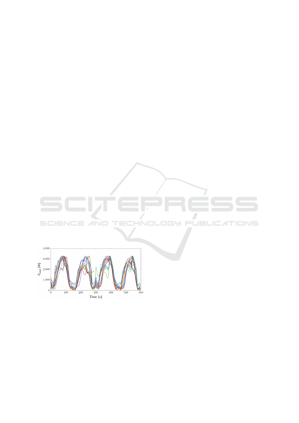
3.3 External Heating Proﬁles

As mentioned previously, the load circuit is heated by

an external heating proﬁle

load

, 10 minutes long, and

consisting of 200 samples. In this paper, we consider

130 different proﬁles, which are based on a public li-

brary for unit commitment, see (IEEE, 2024). 15 of

the proﬁles are shown in Figure 3: it can be seen that

repetitive trends occur, but that still signiﬁcant varia-

tions between the proﬁles are present. In the remainder

of this paper, the ﬁrst 100 proﬁles are selected as the

training set, and the last 30 proﬁles as the test set.

Figure 3: 15 of the 130 heating proﬁles.

4 REINFORCEMENT LEARNING

ENVIRONMENT

We now deﬁne the Markov Decision Process to express

the cooling case as an RL problem, by deﬁning its

action space, observation space and reward function.

4.1 Initial State Distribution

In our setup, episodes have a ﬁxed length of 200 time-

steps, equal to the total task duration. When an episode

terminates, the simulation is reset (the water tempera-

ture in the tank is reset to 25

◦

C, and the 3 chillers are

turned off), and a new simulation can be started.

4.2 Action Space

For the cooling case there are both discrete (on/off)

and continuous actions (if on, at what power level).

To make it easier for the RL, we transform this into

a problem with only continuous actions. Since it is

considered best practice (Rafﬁn et al., 2021) to have

the action and state spaces centered around 0, we chose

a single value to control each chiller, ranging from -1

to 1, which we map to the chiller controls:

• Values below -0.5 are mapped to off.

•

Values between -0.5 and 0 are mapped to on, but

at minimum power input.

•

Positive values are mapped to on, with the range

1] corresponding to [

, P

], with

and

the minimum and maximum chiller power inputs.

This allows the agent to control the on/off status

of the chillers, in addition to their power consumption

setpoints, with a single real value.

4.3 Observation Space

The observation space consists of several values that

measure past tank temperatures and power consump-

tion setpoints. For every time-step, 4 values are logged:

the change of temperature (

(

)

−T

(

k −

1)) of the wa-

ter in the tank during the previous time-step, and the

power input setpoints of the 3 chillers. When produc-

ing observations, the environment looks

time-steps

in the past to produce

real values corresponding

to changes in water temperature at these past

time-

steps. The environment also looks

time-steps in the

past to produce 3

real values corresponding to set-

points of the chillers during these past

time-steps.

and

can be distinct, and in our experiment, we

use

= 10 past temperatures and

= 6 past set-

points. A ﬁnal observation is given to the agent, a

running average (rate of 0.1) of the water temperature.

By observing past changes of water temperatures

and chiller setpoints, the agent is able to learn:

•

The past demand and losses, by comparing the

changes of water temperature with the setpoints.

•

The efﬁciency of the chillers, and how they interact

with the system (the agent has no model and has

to discover the effect of its actions).

Reinforcement Learning for Model-Free Control of a Cooling Network with Uncertain Future Demands

•

All this combined allows the agent to build an

internal estimate of what the future demand may

be, given that the 100 demand proﬁles are distinct

but share some structure.

This information is still not enough for optimal con-

trol, as it does not contain information about the future

demand, but observing a history of past sensor read-

ings has been shown to be one of the best approaches

to learn in Partially Observable MDPs (Bakker, 2001),

and is straightforward to implement.

4.4 Reward Function

In this section, the reward function it explained. The

reward function is the negation of the change in cost

that occurs after a given time-step k ∈ [1, N]. By sum-

ming over all time steps, the total reward (of a given

episode) is computed.

The reward function is build up similarly to the cost

(and temperature constraint) introduced previously in

Section 3.2. Hence, the considered reward function

(for a given time-step) consists of three components:

Minimizing Energy Consumption. The ﬁrst part

of the reward function is equal to (minus) the to-

tal energy consumed during the considered time-

step

, i.e.,

input, total

(

), with

input, total

(

) the

power consumed by all the chillers at sample k.

Penalizing Turning-On of Chillers. The second

part of the reward function is a (negative) turn on

penalty when a chiller turns on, like in Section 3.2.

Constraint Satisfaction. If the constraint on the

water temperature (in this case, set to 25

◦

C) is

violated, a reward of -2 is given to the agent for

this time-step. A backup policy then turns all the

chillers ON to maximum power, thereby also pro-

viding several turn-on penalties. The episode oth-

erwise continues, and the agent learns over time to

meet the constraint to avoid the -2 rewards.

Over an episode (of

samples), after the agent

has learned to always meet the constraint, the sum of

these rewards perfectly corresponds to the actual cost

of running the episode, given by Eq. 3.

4.5 Training Procedure

The RL agent is trained using the Proximal Policy

Optimization (Schulman et al., 2017), as implemented

in Stable-Baselines 3 (Rafﬁn et al., 2021). Hyper-

parameters are given in Section 6. The agent is allowed

to learn for 40 million time-steps (about 5 hours using

8 AMD Zen2 cores running at 4.5 Ghz).

Every 128000 time-steps, the current policy

learned by the agent is saved in a checkpoint ﬁle (of

about 1.7 MB). After training, all these policies are

run on demand proﬁle 1 with exploration disabled, and

the run with the smallest cost is selected as the RL

policy. This evaluation takes about 11 minutes on a

single AMD Zen2 core, and ﬁnds a policy that:

•

Is about 2% better than the last policy produced by

the agent (cost of 446 instead of 455);

•

Was produced after about 20 million time-steps,

so signiﬁcantly before the end of the training (40

million time-steps).

These two points combined indicate that it is both

beneﬁcial and cheap to evaluate a collection of learned

RL policies before picking one to use, because agents

do not monotonically become better as they learn, but

instead oscillate a bit around the optimal policy.

5 BENCHMARK CONTROLLERS

5.1 Model-Predictive Controller

As a ﬁrst benchmark, we use a model-predictive con-

troller (MPC). It optimizes the state trajectories and

controls over a given horizon

mpc

. At every time step

k ∈

, N

], an optimization problem is solved. After

solving, the ﬁrst sample of the computed input se-

quence is then applied to the system, and we again

solve the optimization problem for the next time sam-

ple. This is repeated for the entire horizon with length

. The resulting discrete-time optimization problem

is set up as follows:

minimize

T (·),P

input

(·)

k=1

∑

k=N

mpc

input, total

(k) + (5a)

i=1

∑

i=3

input, previous

− P

input

(1))

s. t. (2) ∀ k ∈ [1, N

mpc

], (5b)

T (k) ≤ 25 ∀ k ∈ [1, N

mpc

], (5c)

≤ P

input

(k) ≤ P

∀ k ∈ [1, N

mpc

], (5d)

T (1) = T

init

. (5e)

Eq. 5a implements the cost function. It is set to mini-

mize (1) the sum of all input power, that is, the total

energy consumption over the entire horizon, along

with (2) a regularization term which penalizes the dif-

ference of the ﬁrst sample of the current horizon and

the last input applied to the system, thereby penaliz-

ing switching the control input. The system dynamics

are implemented using Eq. 2, using multiple shoot-

ing. Eq. 5c implements the constraint on the allowed

ICINCO 2025 - 22nd International Conference on Informatics in Control, Automation and Robotics

temperature, and Eq. 5e ensures each MPC iteration

starts from the temperature last measured on the sys-

tem. Finally, for each chiller, constraints are set on the

allowed input power in Eq. 5d.

As mentioned previously, each chiller can be ON

(and if so, in a speciﬁc input power range), or OFF.

This would cause the MPC to require a mixed-integer

optimization problem, which are harder to solve. In

this paper, we approximate the true mixed-integer prob-

lem by decomposing it using an outer loop (with only

discrete variables) and an inner loop (with only contin-

uous values). Solving the full optimization for a single

time instance can be done using the following steps:

•

Step 1: Select one of the combinatorial options for

ON/OFF status of the 3 chillers e.g., [ON, OFF,

OFF]

•

Step 2: For the option selected in step 1, solve the

inner loop MPC problem that minimizes the total

energy.

•

Step 3: Go back to step 1 and select another com-

binatorial option of chiller ON/OFF statuses, until

all options are computed

•

Step 4: Select the option with the lowest total

energy as the solution to the nested MPC problem

In other words, the outer loop selects which chillers

are ON or OFF (in the entire time interval). Then,

the inner loop solves the above optimization problem

(with input powers kept within to their input ranges for

chillers that are ON, or kept at zero when OFF). The

outer loop iterates over all possible combinations (in

this case 8), and computes the resulting cost according

to Eq. 3. The solution with the lowest cost (that

meets the temperature constraints) is then selected

and applied to the system. Note there is no penalty

included for switching between ON/OFF states in the

inner loop, since the MPC problem solved in the inner

loop assumes the same set of chillers remains ON

during the entire horizon. In the outer loop we do

penalize sets that require a change in ON/OFF states

when compared to the solution at the previous time

sample.

The MPC problem is implemented using

CasADi (Andersson et al., 2019) and is solved using

IPOPT (Biegler and Zavala, 2009).

5.2 Rule-Based Controller

As a second benchmark, we use a rule-based controller

or RBC. It is implemented in the following way:

•

A feedback input

desired

(

set point

− T

) is

computed using a proportional controller with gain

. The setpoint is given by

set point

, which can be

set equal to the constraint on the load temperature

(25

◦

C) minus an offset. This offset can be tuned

to ensure that the controller meets the temperature

constraint for varying heat load proﬁles.

•

From

desired

, we can select which chillers to turn

ON. This is done by ﬁrst inspecting the relative

efﬁciencies of combinations of chillers, as shown

in Fig. 4. Then, for each

desired

, we can select

the most efﬁcient combination. In order to prevent

switching of sets too often, we introduce a simple

deadband (i.e., we only switch between combina-

tions if the difference has exceeded this deadband).

•

After the set of chillers to be used is chosen in

the previous step, we select the input powers of

each chiller. The goal is to match

desired

, while

minimizing the total required input power by the

chillers. This is done via a simple heuristic.

0 500 1,000 1,500 2,000 2,500 3,000 3,500

500

1,000

1,500

cool

[W]

input

[W]

1 2 3 1&2 2&3 1&2&3 1&3

Figure 4: Relative efﬁciencies of the sets of chillers.

6 RESULTS

6.1 Nominal Case

In this section, we have run each of the controllers for

the nominal case: without any perturbations. For each

of the controllers, the settings are as follows:

•

The RL algorithm is based on the Proximal Policy

Optimization algorithm (Schulman et al., 2017),

as implemented in the Stable Baselines 3 (Rafﬁn

et al., 2021). The hyper-parameters of that agent

are the default ones from Stable Baselines 3 (as of

January 2023), with the exception of: 128 paral-

lel environments (n_envs), a batch size of 200, and

both the actor and value networks are feed-forward

neural networks with 2 hidden layers of 256 neu-

rons. Given the limited number of neurons the risk

of overﬁtting was deemed low, but more sparse

neural networks could be explored in future work

to perhaps improve results in regions outside of

training. The RL agent was allowed to learn in our

simulated setup for 40 million time-steps. These

hyper-parameters have been obtained through in-

formed manual tuning, and our results haven been

found to be robust to changes in hyper-parameters.

Reinforcement Learning for Model-Free Control of a Cooling Network with Uncertain Future Demands

•

The MPC has a horizon of

mpc

= 10 samples, the

other parameters are set as outlined earlier.

•

For the RBC, we set the temperature setpoint to

23.1

◦

C and K

= 2500.

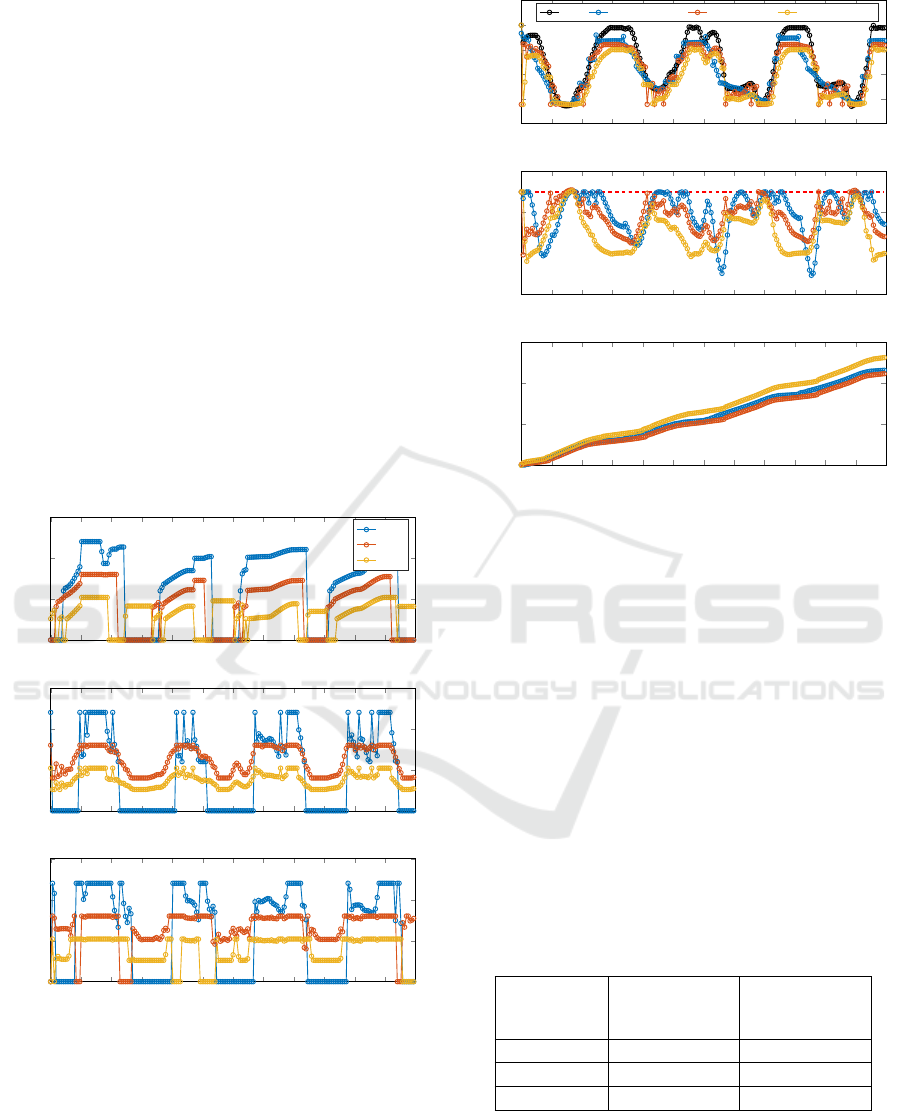
We show the outcome of each of the three con-

trollers for a speciﬁc example scenario in Figure 5

(the control inputs) and Figure 6 (cooling power: de-

mand and delivered, temperature, cost). As can be

seen from the plots, all three make choices that cause

the chillers to turn ON and OFF, and choose the corre-

sponding power input, but the solutions differ between

the controllers. As can also be seen, the provided

cooling for all 3 controllers matches the load proﬁle

somewhat, though not perfectly. This can also be seen

in the achieved temperature, which goes up or down

when the demand isn’t matched exactly (which is al-

lowed as long as the temperature remains below the

upper bound, though there will be more losses if the

temperature is lower). Lastly, it can be seen that the

accumulated cost of the three controllers is similar for

MPC and RL, but signiﬁcantly higher for the RBC.

0 50 100 150 200 250 300 350 400 450 500 550 600

−4,000

−3,000

−2,000

−1,000

1,000

Time [s]

Power [W]

load

cool, total

(MPC) P

cool, total

(RL) P

cool, total

(RBC)

0 50 100 150 200 250 300 350 400 450 500 550 600

22.5

23.5

24.5

25.5

Time [s]

Temperature [deg C]

0 50 100 150 200 250 300 350 400 450 500 550 600

200

400

600

Time [s]

Cost function J

0 50 100 150 200 250 300 350 400 450 500 550 600

250

500

750

Time [s]

input

[W]

MPC

input

0 50 100 150 200 250 300 350 400 450 500 550 600

250

500

750

Time [s]

input

[W]

0 50 100 150 200 250 300 350 400 450 500 550 600

250

500

750

Time [s]

input

[W]

RBC

Figure 5: Outcome with each of the 3 controllers on a nomi-

nal example scenario. The plots show the electrical powers

for all 3 chillers, ﬁrst for MPC, then for RL, and ﬁnally for

RBC.

We have also averaged the results, over both train-

ing and test set, as shown in Table 1. Similar obser-

vations can be made regarding MPC and RL signiﬁ-

cantly beating the RBC. The RL even appears to have

a lower cost than MPC, but an exact comparison is

0 50 100 150 200 250 300 350 400 450 500 550 600

−4,000

−3,000

−2,000

−1,000

1,000

Time [s]

Power [W]

load

cool, total

(MPC) P

cool, total

(RL) P

cool, total

(RBC)

0 50 100 150 200 250 300 350 400 450 500 550 600

22.5

23.5

24.5

25.5

Time [s]

Temperature [deg C]

0 50 100 150 200 250 300 350 400 450 500 550 600

200

400

600

Time [s]

Cost function J

0 50 100 150 200 250 300 350 400 450 500 550 600

250

500

750

Time [s]

input

[W]

MPC

input

0 50 100 150 200 250 300 350 400 450 500 550 600

250

500

750

Time [s]

input

[W]

0 50 100 150 200 250 300 350 400 450 500 550 600

250

500

750

Time [s]

input

[W]

RBC

Figure 6: Outcome with each of the 3 controllers on a nomi-

nal example scenario. The plots show for all 3 controllers

the resulting cooling power versus the demand, the resulting

temperature (including the setpoint of 25

◦

C (red dashed

line), and the corresponding accumulated cost.

hard since the RL did slightly violate the upper bound

on the temperature (by 0.05

◦

C), which the MPC did

not. Based on rough analysis, this is not expected to

yield more than 1% of difference in energy cost, after

the RL would be retrained with a small temperature

constraints margin. So we conclude the RL achieves

nearly the same performance as the MPC does.

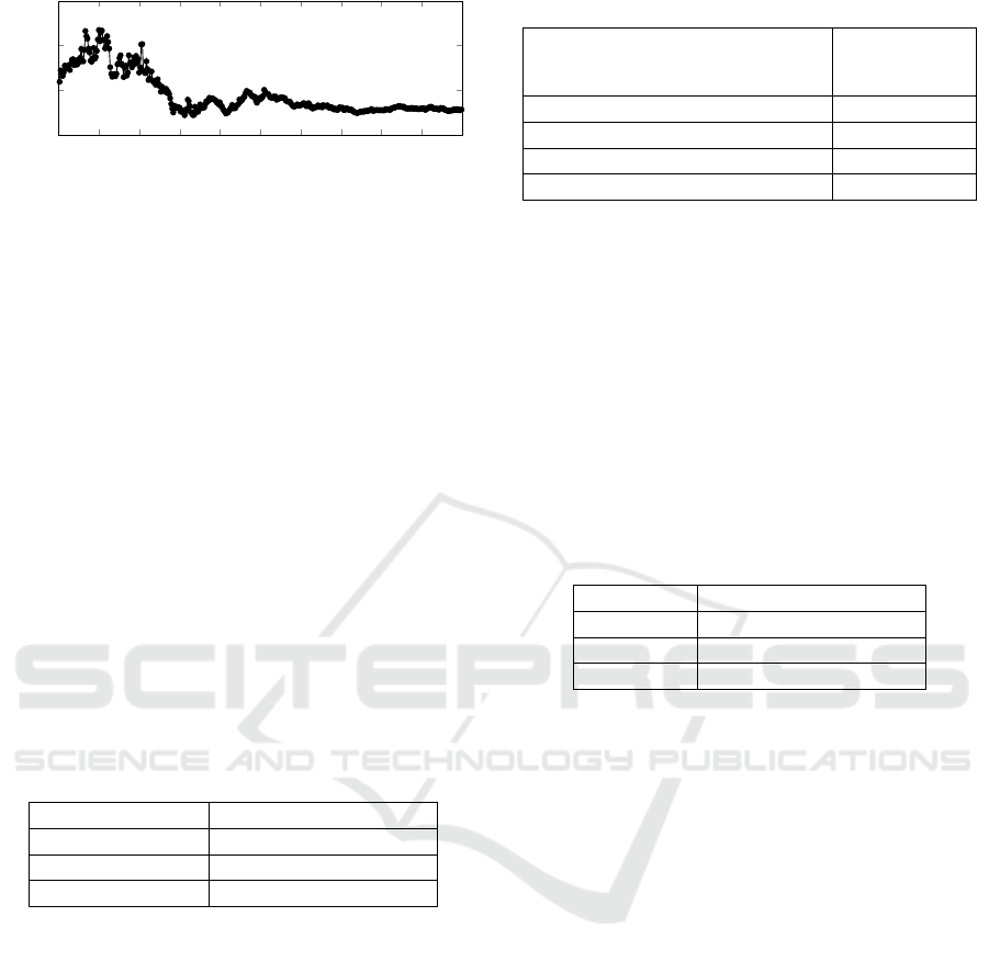
The results shown for the RL are those achieved af-

ter it has learned how to control the chillers effectively.

Figure 7 shows the evolution of the performance from

the initial stages of the learning, until the ﬁnal con-

troller whose results were shown in the graph and the

table.

Table 1: Performance for the nominal case.

Algorithm

Average cost

(train set)

Average cost

(test set)

MPC 454 J 450 J

RL 450 J 448 J

RBC 517 J 512 J

6.2 MPC with Shorter Predictions

In this section, we analyse what happens when the

MPC is given shorter prediction windows, in this case

ICINCO 2025 - 22nd International Conference on Informatics in Control, Automation and Robotics

0.5

1.5

2.5

3.5

4.5 5

·10

400

500

600

700

Time steps

Average cost

Figure 7: Improvement of the RL policy during the training

process (50M time samples, 5:30 hours in simulation). The

agent already learns a good policy at around 20M samples,

and then further stabilizes.

4 samples (i.e., 12s, so short in comparison with the

period time of load variations or the system time con-

stant). The RBC and the RL do not use predictions, so

achieve the same results in the previous section.

The results are shown in Table 2. Therein we can

see that the MPC with shorter predictions has a per-

formance that falls below that of the RL. We did not

include an MPC with even shorter predictions, or none

at all, since these often violate the temperature con-

straints, and therefore would require more extensive

tuning.

This shows that the MPC needs to have good pre-

dictions, over a sufﬁciently long window, to be able to

control optimally. And since the RL performs equiv-

alently to the MPC controller with good predictions,

it furter shows that even though the RL does not use

predictions explicitly, it has learned how to implicitly

anticipate to the types of proﬁles in the training set.

Table 2: Impact of shorter predictions.

Algorithm Average cost (test set)

MPC (4 samples) 475 J

RL 448 J

RBC 512 J

6.3 MPC with Imperfect Predictions

In this section, the MPC is provided with predictions

that overestimate or underestimate the demand by 10%,

in an attempt to study real-world behavior when pre-

dictions of future demand are imperfect. Again, for

the RL and the RBC the results are the same. It can

be seen in Table 3 that the MPC is sensitive to these

predictions, and that in case of such mismatch the RL

performs better than the MPC.

6.4 RL with Demands Beyond Training

Finally, we consider the scenario where the demands

encountered are different to those considered during

the training. This to study the effect on the RL: not of

Table 3: Impact of imperfect predictions.

Algorithm

Average cost

(test set)

MPC (demand over-estimated) 490 J

MPC (demand under-estimated) 519 J

RL 448 J

RBC 512 J

having imperfect predictions since the RL does not use

them, but of having a training set that is not complete,

or not fully representative of real world behavior.

Here we have scaled down the demands by a factor

0.8, while the controllers are kept the same as in the

previous case. This has an impact on the RL, since the

patterns that are implicitly being exploited no longer

correspond to those faced. The MPC on the other hand

is given this new demand proﬁle, and can therefore ad-

just very effectively. As a result, the RL now performs

noticeably less performant than the MPC controller, as

seen in Table 4.

Table 4: Impact with scaled down demands.

Algorithm Average cost (test set)

MPC 380 J

RL 391 J

RBC 463 J

6.5 Training and Runtime

While the RL has achieved good results, it did require

a learning process to do so, running 200000 episodes

(40M time samples) of the simulation model. This

took around 5 hours using 8 AMD Zen2 cores running

at 4.5 Ghz. This is still signiﬁcantly shorter than the

engineering time needed to work out the approaches,

set up the environments and debug the codes, for both

MPC and RL. Training time is thus not yet the real bot-

tleneck. In future cases, when more variations are con-

sidered, or model-plant mismatch, this number might

increase further however, so care will need to be taken

to keep this manageable.

We also evaluated the runtime needed to evaluate or

execute the controllers. As shown in Table 5, the MPC

required on average a calculation time of 0.50 seconds,

and the RL 0.04 seconds. This is a signiﬁcant advan-

tage of using the RL over the MPC controller. Note

that there are various ways to reduce the computation

time of an MPC e.g., reduce its control horizon, use a

move-blocking implementation, increase its sampling

rate, change low-level optimizer types and settings, but

these are not the focus of this work.

Reinforcement Learning for Model-Free Control of a Cooling Network with Uncertain Future Demands

Table 5: Calculation times.

MPC 0.5 s

RL 0.04 s

7 DISCUSSION

From the previous, we can see that in nominal con-

ditions RL can match the performance of a nearly-

optimal MPC controller. However, RL does so without

using predictions of upcoming demands (nor models),

which the MPC does use. Furthermore, since the RL

does better than an MPC with a reduced prediction

horizons, we can see that the RL has implicitly learned

the typical demand patterns, and achieves MPC-like

performance without needing predictions of the fu-

ture demands explicitly. This ﬁts with the observation

that when we use demands outside of the training set,

the performance of the RL does degrade, as then the

implicitly learned patterns are no longer correct.

For industrial usage there is then a trade-off to be

made. Beyond savings in runtime calculations, using

RL would have the beneﬁt of not needing good predic-

tions of future demands, as even with small prediction

imperfections the MPC performance drops below the

RL. On the other hand, this only holds when the train-

ing data for the RL is sufﬁciently rich to ensure that

the usage patterns faced during operation fall within

the implicitly learned behavior. In future work we will

study this further. We will study if we can train an RL

for a more diverse set of usage patterns (e.g., includ-

ing rescaled versions) and initial system states (e.g.,

initial tank water temperatures) and how much the per-

formance degrades when the increased variety makes

it harder to ﬁnd patterns to exploit. Techniques such

as domain randomization (Tobin et al., 2017) might

prove helpful in this case. Furthermore, investigations

into possible overﬁtting due to fully-connected neural

networks should be addressed, and possibly resolved

with more sparse networks. Another interesting option

for study is combining both approaches: let the RL

learn patterns implicitly, but also provide it explicit

predictions, though possibly indirect or imperfect.

It also has to be noted that while we focused on

the impact of imperfect predictions of future demands

in this paper, a practical challenge that will be faced

in reality is that the models describing the system dy-

namics will also be imperfect. This will impact the

MPC which uses them explicitly, but it will also im-

pact the RL which uses the models to run simulations

to train on. Studying the impact of imperfect models is

a very interesting challenge, which we will also tackle

in future work. We plan to study training RL on sets

of variant models, increasing its robustness, and/or ap-

proaches wherein we allow a limited ﬁne-tuning of the

RL once deployment to the real plant occurs. Next to

that, combinations of RL methods with other methods

like MPC or RBC controllers will also be considered.

Beyond using RL or combining it with other meth-

ods, an alternative (yet CPU intensive) solution is to

improve the MPC to better handle imperfect predic-

tions and models, using robust, stochastic or multi-

stage formulations. We did not do so or tune the MPC

extensively in this paper, since our goal was to show

the MPC relies on predictions, whereas the RL did not.

8 CONCLUSION

This paper compares several controllers on a simu-

lated cooling system with 3 chillers. The proposed

RL achieves a performance nearly equal to that of

an MPC, but without explicit demand predictions nor

model, and at a reduced computational cost. It does

lose some performance when demands outside the

training set are used, but the MPC loses performance

when the predicted demands lose accuracy. Future

work will therefore focus on making the RL robust

to more diverse usage patterns, by e.g. making them

rely on both implicitly learned patterns and explicit

predictions. We will further study how to train RL

on imperfect models, and how to ensure an efﬁcient

transfer is possible when there is mismatch between

simulation environment and reality.

This paper implemented the proposed approach to

a single use-case with a simulation of a scaled-down

industrial usage pattern. Nevertheless, losses have

been rescaled in order to make the outcomes repre-

sentative for a wider range of problems: those where

complex systems (multiple units, non-linear behavior,

mixed integer controls) need to be controlled, while

balancing short and long term cost drivers (inability

to switch active units all the time requiring to look

further ahead and anticipate, while considering the im-

pact of losses as a function of the states encountered).

We expect similar outcomes and trade-offs to hold for

many industrial cases with similar properties, like unit

commitment problems, industrial cooling, water treat-

ment, pumping plants, heating networks, compressed

air generation, etc. It is still an open question which of

the methods will be more realistic when the number of

controllable degrees of freedom increases, e.g. when

a pumping plant with 20 pumps is faced rather than

one with 3. The challenge will be to let the RL ﬁnd

solutions in an acceptable period of training time. On

the other hand, for the MPC mostly the runtime will

become a bottleneck, as the MPC with our current

formulation scales quadratically in the inner loop (in

ICINCO 2025 - 22nd International Conference on Informatics in Control, Automation and Robotics

ideal case, in practice worse due to non-linearities),

but combinatorially in the outer loop. However, sev-

eral other formulations exist in literature, including

heuristic methods, that keep it tractable up to 20+ con-

trollable units.

BROADER IMPACT STATEMENT

Our contributions make more industrial machines con-

trollable in an autonomous way. We mainly envi-

sion positive impacts on society, such as reduced en-

ergy consumption for the same manufacturing quality,

higher manufacturing quality (less waste) and a gen-

eral improved economy. The machines that would

beneﬁt from our contribution are usually not directly

controlled by people, so we don’t expect jobs to be

lost to automation with our contribution. We however

acknowledge that any improvement in automation also

improves it for sensitive use, such as military equip-

ment production.

ACKNOWLEDGMENTS

This research is done in the framework

of the Flanders AI Research Program

(https://www.ﬂandersairesearch.be/en) that is ﬁ-

nanced by EWI (Economie Wetenschap & Innovatie),

and Flanders Make (https://www.ﬂandersmake.be/en),

the strategic research Centre for the Manufacturing

Industry, who owns the Demand Driven Use Case.

The authors would like to thank everybody who

contributed with any inputs to make this publication.

REFERENCES

Andersson, J. A., Gillis, J., Horn, G., Rawlings, J. B., and

Diehl, M. (2019). Casadi: a software framework for

nonlinear optimization and optimal control. Mathemat-

ical Programming Computation, 11(1):1–36.

Asadi, K., Parikh, N., Parr, R. E., Konidaris, G. D., and

Littman, M. L. (2021). Deep radial-basis value func-

tions for continuous control. In Proceedings of the

AAAI Conference on Artiﬁcial Intelligence, volume 35,

pages 6696–6704.

Bakker, B. (2001). Reinforcement learning with long short-

term memory. Advances in neural information process-

ing systems, 14.

Biegler, L. T. and Zavala, V. M. (2009). Large-scale nonlin-

ear programming using ipopt: An integrating frame-

work for enterprise-wide dynamic optimization. Com-

puters & Chemical Engineering, 33(3):575–582.

Borase, R. P., Maghade, D., Sondkar, S., and Pawar, S.

(2021). A review of pid control, tuning methods and

applications. International Journal of Dynamics and

Control, 9:818–827.

Camacho, E. F. and Alba, C. B. (2013). Model predictive

control. Springer science & business media.

Chen, R., Lan, F., and Wang, J. (2024). Intelligent pressure

switching control method for air compressor group

control based on multi-agent reinforcement learning.

Journal of Intelligent & Fuzzy Systems, 46(1):2109–

2122.

De Somer, O., Soares, A., Vanthournout, K., Spiessens, F.,

Kuijpers, T., and Vossen, K. (2017). Using reinforce-

ment learning for demand response of domestic hot

water buffers: A real-life demonstration. In 2017 IEEE

PES Innovative Smart Grid Technologies Conference

Europe (ISGT-Europe), pages 1–7. IEEE.

Frank, R. J., Davey, N., and Hunt, S. P. (2001). Time series

prediction and neural networks. Journal of intelligent

and robotic systems, 31:91–103.

Fujimoto, S., Hoof, H., and Meger, D. (2018). Addressing

function approximation error in actor-critic methods.

In International conference on machine learning, pages

1587–1596. PMLR.

Glover, K. (2021). H-inﬁnity control. In Encyclopedia of

systems and control, pages 896–902. Springer.

Haarnoja, T., Zhou, A., Hartikainen, K., Tucker, G., Ha, S.,

Tan, J., Kumar, V., Zhu, H., Gupta, A., Abbeel, P., et al.

(2018). Soft actor-critic algorithms and applications.

arXiv preprint arXiv:1812.05905.

Hessel, M., Modayil, J., Van Hasselt, H., Schaul, T., Ostro-

vski, G., Dabney, W., Horgan, D., Piot, B., Azar, M.,

and Silver, D. (2018). Rainbow: Combining improve-

ments in deep reinforcement learning. In Proceedings

of the AAAI conference on artiﬁcial intelligence, vol-

ume 32.

IEEE (2024). Ieee pes power grid benchmarks.

Lewis, F. L., Vrabie, D., and Syrmos, V. L. (2012). Optimal

control. John Wiley & Sons.

López-Ibáñez, M., Prasad, T. D., and Paechter, B. (2008).

Ant colony optimization for optimal control of pumps

in water distribution networks. Journal of water re-

sources planning and management, 134(4):337–346.

Lourenço, H. R., Martin, O. C., and Stützle, T. (2019). Iter-

ated local search: Framework and applications. Hand-

book of metaheuristics, pages 129–168.

Luo, J., Paduraru, C., Voicu, O., Chervonyi, Y., Munns,

S., Li, J., Qian, C., Dutta, P., Davis, J. Q., Wu, N.,

et al. (2022). Controlling commercial cooling sys-

tems using reinforcement learning. arXiv preprint

arXiv:2211.07357.

Mehra, R. and Davis, R. (1972). A generalized gradient

method for optimal control problems with inequality

constraints and singular arcs. IEEE Transactions on

Automatic Control, 17(1):69–79.

Meinhold, R. J. and Singpurwalla, N. D. (1983). Under-

standing the kalman ﬁlter. The American Statistician,

37(2):123–127.

Michalewicz, Z., Janikow, C. Z., and Krawczyk, J. B. (1992).

A modiﬁed genetic algorithm for optimal control prob-

Reinforcement Learning for Model-Free Control of a Cooling Network with Uncertain Future Demands

lems. Computers & Mathematics with Applications,

23(12):83–94.

Mnih, V., Kavukcuoglu, K., Silver, D., Rusu, A. A., Veness,

J., Bellemare, M. G., Graves, A., Riedmiller, M., Fidje-

land, A. K., Ostrovski, G., et al. (2015). Human-level

control through deep reinforcement learning. nature,

518(7540):529–533.

Monahan, G. E. (1982). State of the art—a survey of partially

observable markov decision processes: theory, models,

and algorithms. Management science, 28(1):1–16.

Rafﬁn, A., Hill, A., Gleave, A., Kanervisto, A., Ernestus, M.,

and Dormann, N. (2021). Stable-baselines3: Reliable

reinforcement learning implementations. The Journal

of Machine Learning Research, 22(1):12348–12355.

Roy, N. and Gordon, G. J. (2002). Exponential family pca

for belief compression in pomdps. Advances in Neural

Information Processing Systems, 15.

Schulman, J., Levine, S., Abbeel, P., Jordan, M., and Moritz,

P. (2015). Trust region policy optimization. In In-

ternational conference on machine learning, pages

1889–1897. PMLR.

Schulman, J., Wolski, F., Dhariwal, P., Radford, A., and

Klimov, O. (2017). Proximal policy optimization algo-

rithms. arXiv preprint arXiv:1707.06347.

Shang, W., Wang, X., Srinivas, A., Rajeswaran, A., Gao,

Y., Abbeel, P., and Laskin, M. (2021). Reinforcement

learning with latent ﬂow. Advances in Neural Informa-

tion Processing Systems, 34:22171–22183.

Silver, D., Lever, G., Heess, N., Degris, T., Wierstra, D., and

Riedmiller, M. (2014). Deterministic policy gradient

algorithms. In International conference on machine

learning, pages 387–395. Pmlr.

Sutton, R. S., McAllester, D., Singh, S., and Mansour, Y.

(1999). Policy gradient methods for reinforcement

learning with function approximation. Advances in

neural information processing systems, 12.

Tobin, J., Fong, R., Ray, A., Schneider, J., Zaremba, W., and

Abbeel, P. (2017). Domain randomization for trans-

ferring deep neural networks from simulation to the

real world. In 2017 IEEE/RSJ international conference

on intelligent robots and systems (IROS), pages 23–30.

IEEE.

Van Hasselt, H. and Wiering, M. A. (2007). Reinforcement

learning in continuous action spaces. In 2007 IEEE

International Symposium on Approximate Dynamic

Programming and Reinforcement Learning, pages 272–

279. IEEE.

Watkins, C. J. and Dayan, P. (1992). Q-learning. Machine

learning, 8:279–292.

Williams, R. J. (1992). Simple statistical gradient-following

algorithms for connectionist reinforcement learning.

Reinforcement learning, pages 5–32.

Zhan, X., Xu, H., Zhang, Y., Zhu, X., Yin, H., and Zheng,

Y. (2022). Deepthermal: Combustion optimization

for thermal power generating units using ofﬂine re-

inforcement learning. In Proceedings of the AAAI

Conference on Artiﬁcial Intelligence, volume 36, pages

4680–4688.

ICINCO 2025 - 22nd International Conference on Informatics in Control, Automation and Robotics