Towards Universal Detection and Localization of Mating Parts in

Robotics

Stefan Marx

, Attique Bashir

2 a

and Rainer M

uller

1 b

Chair of Assembly Systems, Saarland University, Saarbr

ucken, Germany

Department of Assembly Systems, center for Mechatronics and Automation Technology gGmbH, Saarbr

ucken, Germany

Keywords:

Robotics, Assembly, Joining, Object Detection, Geometric Shapes.

Abstract:

A key task in robotics is the precise joining of two components. This approach focuses on detecting basic

geometric shapes such as rectangles, triangles, and circles, etc. on the respective mating counterparts. This

paper ﬁrst examines how precisely individual geometric shapes can be localized using stereoscopy with a sin-

gle camera on the robot arm. After the localization of the individual shapes, the spatial relationships between

these shapes are analyzed and then compared with those of a possible joining partner. If several features

match, transformation parameters are calculated to deﬁne the optimal alignment for an accurate and efﬁcient

assembly. This method emphasizes simplicity and effectiveness in identifying complementary geometries for

precise positioning during assembly tasks.

1 INTRODUCTION

Across a wide range of industries, from automotive to

consumer electronics and medical technology, joining

operations such as plugging, clipping, or pressing are

essential steps in product assembly. Although these

processes are often repetitive and geometrically well-

deﬁned, many of them are still carried out manually.

This is particularly evident in the insertion of electri-

cal connectors, cable harness assembly, and the me-

chanical joining of plastic or metal components. The

underlying reason lies in the complexity of ﬂexible

automation: small variances in part geometry, orien-

tation, or tolerance often require human adaptability,

something traditional robotic systems have struggled

to replicate.

At the same time, several key trends are accel-

erating the push toward robotic solutions. The on-

going shortage of skilled workers, driven by demo-

graphic change and the rising cost of labor, is putting

pressure on manufacturers to automate even low- to

mid-complexity tasks. The growing adoption of elec-

tric vehicles and the digitalization of machinery lead

to an increasing number of connectors and interface

points, many of which require precise positioning and

certain process forces during assembly. Furthermore,

the trend toward mass customization and high product

variability requires ﬂexible, adaptable systems capa-

https://orcid.org/0009-0001-7708-2863

https://orcid.org/0000-0001-9470-556X

ble of handling different joining geometries without

extensive retooling.

Modern robotics, enhanced by vision systems and

sensor integration, is increasingly capable of meeting

these demands. Recent advances in camera-based lo-

calization, force-feedback control, and AI-driven fea-

ture detection allow robots to adapt to slight variations

in components and reliably perform joining tasks that

were previously the domain of human workers. A

particularly promising approach lies in the geometric

analysis of joining partners, more precisely to identify

and match features such as holes, edges, and contours

to determine the correct spatial alignment.

The present work builds upon this idea by propos-

ing a method for the visual detection and analysis of

basic geometric shapes on joining counterparts, us-

ing a single camera mounted on the robot arm. By

evaluating spatial relationships between these shapes

and comparing them across components, it becomes

possible to determine the correct transformation for

precise alignment and assembly. This geometric rea-

soning forms the basis for a lightweight, ﬂexible, and

scalable solution for automated joining tasks in a wide

variety of industrial contexts.

The paper is structured as follows: First, the state-

of-the-art and selected approaches to the generalized

detection of joining partners and the automation of

difﬁcult joining processes with robots are considered.

This is followed by a presentation of the methods con-

sidered here. Subsequently, the detection and local-

ization of geometric shapes is discussed in more de-

Marx, S., Bashir, A. and Müller, R.

Towards Universal Detection and Localization of Mating Parts in Robotics.

DOI: 10.5220/0013707400003982

Paper published under CC license (CC BY-NC-ND 4.0)

In Proceedings of the 22nd International Conference on Informatics in Control, Automation and Robotics (ICINCO 2025) - Volume 2, pages 235-242

ISBN: 978-989-758-770-2; ISSN: 2184-2809

235

tail, and an accuracy analysis is presented. This is fol-

lowed by a summary and an outlook on future work.

2 STATE OF THE ART

In industrial robotics, it is a key challenge for a robot

to automatically recognize where components are lo-

cated and how they are aligned to properly join them.

In this chapter, we provide an overview of the cur-

rent technical approaches to how robots recognize and

localize single components and identify joining part-

ners.

In the past, such tasks were mainly solved using

CAD models. The robot searches for the model in the

camera view and calculates the position of the real ob-

ject. Algorithms such as Iterative Closest Point (ICP)

are used here (Xiang et al., 2017). Such methods can

be very accurate, but require good camera data and of-

ten only work if the object is not obscured or rotated.

In addition, it is cumbersome to model each new part

ﬁrst.

In recent years, methods that work with artiﬁcial

intelligence (AI) and normal camera images (RGB)

have become established. A neural network learns

from many sample images to recognize objects and

predict their orientation (position and rotation). Well-

known approaches such as PoseCNN (Xiang et al.,

2017) or YOLO-6D (Tekin et al., 2018) work directly

with images and can thus identify speciﬁc compo-

nents. Newer models such as ZebraPose (Su et al.,

2022) also try to deal with hidden or difﬁcult to distin-

guish parts. The problem with this is that these meth-

ods usually only work with previously known objects.

If a new part is added, such as a different type of con-

nector, the system often has to be retrained. This is a

major obstacle for ﬂexible assembly systems.

Another approach focuses less on the concrete

“recognition” of an object and more on shapes:

Holes, edges, cylinders, surfaces. Systems such as

PVNet (Peng et al., 2019) or EPOS (Hodan et al.,

2020) analyze such features in the image and derive

the position of the object from them. This also works

well if, for example, the object is symmetrical or par-

tially obscured. Methods such as SurfEmb (Haugaard

and Buch, 2022), which learn a kind of “ﬁngerprint”

of the surface - regardless of the speciﬁc object - are

particularly interesting here. This way of thinking ﬁts

well with our goal: instead of recognizing speciﬁc

parts, we want to use general geometric features to

ﬁnd out which parts ﬁt together in principle.

Instead of relying solely on 2D camera im-

ages, many systems today combine color information

(RGB) with depth data. Such RGB-D systems use

a depth camera, for example, as in Microsoft Azure

Kinect DK. Methods such as DenseFusion (Wang

et al., 2019a) and MoreFusion (Wada et al., 2020)

combine both types of information to achieve more

precise results - even in difﬁcult lighting conditions

or when parts overlap.

Completely new methods go one step further: they

try not only to recognize a speciﬁc part, but also to

understand what type of component it belongs to -

for example: “This is a cylindrical plug” or “a round

opening”. One example of this is the NOCS sys-

tem (Wang et al., 2019b), which introduces a type of

neutral coordinate shape that can be used to recognize

any object within a category (e.g. “bottles”). Fur-

ther developments such as FS-Net (Liu et al., 2019)

or SPD (Irshad et al., 2022) show that it is possible

to recognize new variants with just a few training ex-

amples. This is a major advance for applications in

which the components change frequently - in ﬂexible

production lines, for example.

Other methods deal directly and very speciﬁcally

with identifying joining partners. In (Kuo et al.,

2019) potential joining positions on printed circuit

boards are identiﬁed and then matched on the basis

of structural relationships to the components. With

Form2Fit (Zakka et al., 2020), a framework was

developed that learns general guidelines for shape

matching between joining partners in order to solve

problems, for example, when packaging goods. How-

ever, the system is limited to two-dimensional space

and requires the joining partners to lie ﬂat on a work

surface.

Research is clearly moving in one direction: away

from rigid, model-based systems and towards ﬂexi-

ble, learning-based processes that can also deal with

unknown or slightly modiﬁed components.

In the next chapter, we show how our own ap-

proach picks up on these developments and combines

them with a novel method: We analyze the geomet-

ric shapes found on components directly in the sen-

sor data to make universal statements about which

parts ﬁt together, regardless of what they are called

or which product family they come from.

3 METHOD

Our method for automated recognition and joining of

two related components can be divided into the fol-

lowing steps (see Figure 1): It starts with image ac-

quisition. For this purpose, stereo image pairs of the

scenes in which the two matching joining parts are

assumed to be located are recorded. In the second

step, geometric shapes such as circles, rectangles, tri-

ICINCO 2025 - 22nd International Conference on Informatics in Control, Automation and Robotics

236

angles etc. are then searched for in the images. This

is followed by the localization of the shapes in space.

The shapes found in a scene are then placed in rela-

tion to each other before the features of both scenes

are matched. If different features are successfully

matched, a set is created, and a position and orien-

tation in space is determined. This is followed by the

robot picking up a joining partner and the actual join-

ing process. As the accuracy achieved in the local-

ization of the components is sometimes worse than

the joining tolerances, the joining is carried out us-

ing force-controlled application. The grasping of a

joining partner and the actual joining have not been

implemented at the time of publication. The focus of

this paper is on the description of the general method

and on the proof of sufﬁcient accuracy in the localiza-

tion of the geometric shapes.

The previously described ﬂow is the intended pro-

cess in the event that the relevant sides of the join-

ing partners can be captured very well with a cam-

era mounted on the robot. However, the aim of the

method is also to be able to automatically join elec-

trical plug connections, such as the high-voltage plug

in Figure 2. Here it can be assumed that the plugs are

placed on a table, lying in a box or hanging. As a re-

sult, it is possible that the end faces relevant for join-

ing cannot be observed very well using stereoscopy

and a good viewing angle. Therefore, the method

should be adapted later as follows: (see Figure 2).

First, a possible connector in the working area is to

be identiﬁed using object recognition and a simple

gripping pose for picking up the connector is to be

determined. After the robot has picked up the con-

nector using a simple two-jaw gripper, the connector

is held in front of a static camera to identify further

features on the front side using the principle of stere-

oscopy. As described above, the feature sets are ﬁrst

determined as well as the position of these sets in re-

lation to the gripper TCP. This is to compensate for

inaccurate gripping or picking up of the connector at

the start of the process. The connector socket is then

localized using a camera mounted on the robot, again

using stereo image pairs.

To detect and pick up a plug, further object recog-

nition is necessary. This would limit the general valid-

ity of the method, although there are already promis-

ing approaches to recognizing a large number of dif-

ferent plugs (Wang and Johansson, 2023).

3.1 Image Aquisition, Detection and

Localization

For this purpose, a 2D camera mounted on a robot

arm takes two images of the scene from different an-

Image

Aquisition

Object

Detection

Single

Object

Localization

Feature

Matching

Feature Set

Localization

Force

controlled

Joining

Figure 1: Summary of the method presented in this paper.

gles, in which the two matching joining parts are as-

sumed to be located. Along with the stereo image

pairs, the robot’s respective positions are also read out

and stored. Object recognition is then performed us-

ing a YOLOv11 instance segmentation model. This

model was trained using two-dimensional printouts of

the shapes and three-dimensional objects, where only

the front surface was labelled. The object recognition

results are masks that are subsequently used to de-

termine the centers of the geometric shapes in image

coordinates. Next, the center points are triangulated

using the stereo image pairs, and the center point co-

ordinates are transformed into the robot base coordi-

nate system. The accuracy of this localisation process

is examined in more detail in the following chapter, as

high accuracy is crucial for subsequent matching and

joining processes.

3.2 Feature Matching

Once the individual geometric shapes have been iden-

tiﬁed and located in their respective scenes, they must

be related to each other. Based on the established

relationships, similarities between the two recorded

scenes are analyzed. The following procedure is uti-

lized for this purpose: For each scene, all possible sets

consisting of three objects/centers are formed (see

Figure 3). These sets are then compared between the

scenes and those with the same combinations of geo-

metric shapes are ﬁltered out. This reduces the search

space for the subsequent analysis, which initially in-

volves calculating the connection vectors r

i,i+1

be-

tween all centre points in each set of three. Then,

always starting from one object/center point, the con-

nection vectors to the other two center points are com-

bined with the cross product of the two vectors to

form a non-rectangular coordinate system (Figure 3).

For a set consisting of a square S, a circle C and a tri-

angle T, for example, the following coordinate system

can be formed starting from the square:

= r

C,S

× r

T,S

(1)

= (r

C,S

, r

T,S

, n

) (2)

In the case of three different object shapes (e.g.

square, circle, triangle), it is sufﬁcient to determine

Towards Universal Detection and Localization of Mating Parts in Robotics

237

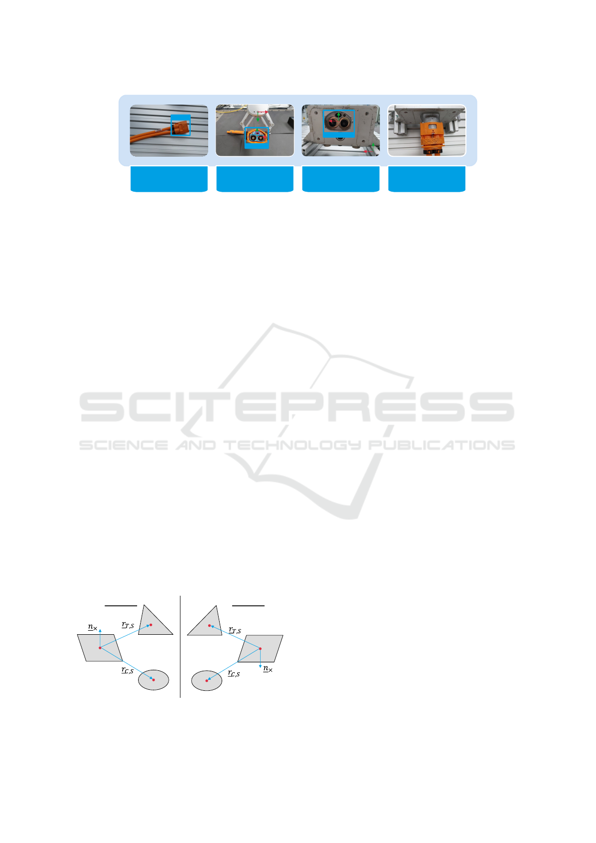
Socket HVR200

Plug HVR200

Plug

DetectPlug Feature Detection

andGraspPosition

Socket Localication JoiningProcess

Plug HVR200

Figure 2: Method sequence for electrical plug connections.

one coordinate system in order to be able to create a

clear comparison with a corresponding set from the

second scene. It should be considered that these two

coordinate systems are created according to the same

principle or the same sequence of vectors. For sets

with two identical shapes, at least two such coordi-

nate systems must be determined; for three identi-

cal shapes, as many as six coordinate systems are re-

quired for the comparison. Three combinations are

created by selecting the “origin” of the coordinate

system and there are two sequences for forming the

cross product for each origin.

To make the comparison, the general transforma-

tions M between the two coordinate systems are cal-

culated.

M = C

)

−1

(3)

If the two coordinate systems match, M should

fulﬁll the criteria of a rotation matrix: The determi-

nant of M must therefore be det(M) = 1. In addi-

tion, the following matrix equation must be fulﬁlled:

M = I where I corresponds to the unit matrix.

Due to the way in which the coordinate systems are

constructed, the relationships of mirrored center point

constellations can also be described with a rotation

matrix. This becomes clear, for example, if the coor-

dinate system in scene 1 in Figure 2 is mentally ro-

tated by 180° around the line drawn between the two

scenes.

For matching sets consisting of three different

shapes, the comparison is unambiguous with only one

pair of coordinate systems. Both coordinate systems

Scene 2Scene 1

Figure 3: Schematic representation of the coordinate sys-

tems for sets of three different shapes.

can be created from the same vector sequence, and a

rotation should be detectable.

For sets with two identical shapes, a total of four

pairs of coordinates can be compared, whereby two

pairs are sufﬁcient to achieve a clear result. The ori-

gin of the coordinate systems is selected in the form

that only exists once. For one scene, two coordi-

nate systems are created using the two possible vec-

tor sequences to form the cross product, which are

then compared with a coordinate system in the second

scene. The determinant can take the value 1 for both

pairs. On the other hand, the matrix product M

should only result in the unit matrix in one case. As an

additional criterion, a length comparison of the con-

nection vectors according to their order in the matri-

ces C

and C

can also be used.

For sets with three identical shapes, a total of 12

coordinate systems can be compared with each other,

as 6 different vector sequences can be constructed for

each scene to calculate the cross product and thus 6

different coordinate systems. Again, it is also suf-

ﬁcient to compare one coordinate system of a scene

with the six of the second scene.

Due to the inaccuracies in the determination of

the center point coordinates, the tests for a rotation

matrix on the real system will not be as unambigu-

ous as described above. It is therefore necessary to

deﬁne certain tolerance limits around the target val-

ues when determining the determinate and the matrix

product. However, the values for these tolerance lim-

its still have to be determined in further experiments.

4 ACCURACY OF THE

LOCALIZATION

As described in the previous chapter, the geomet-

ric shapes are localized using triangulation based on

stereo image pairs. Only a single 2D camera mounted

on the robot end effector is used to record the stereo

images. Different viewing angles can be set by mov-

ing the robot. Due to the time delay between two im-

ages, this type of stereoscopy only allows the obser-

ICINCO 2025 - 22nd International Conference on Informatics in Control, Automation and Robotics

238

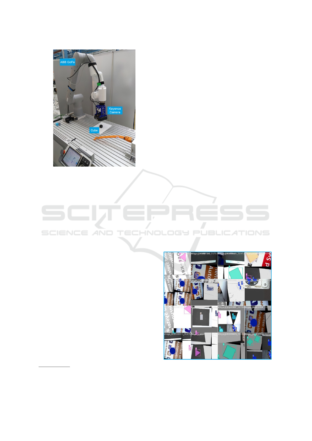
Figure 4: Setup for the accuracy analysis.

vation of static scenes. Further details on the method-

ology can be found in (Marx et al., 2024). In (Marx

et al., 2024) we have shown that using a Kuka Lbr

iiwa and an Intel Realsense D435, accuracies of 2.436

mm with a standard deviation of 0.665 mm can theo-

retically be achieved with this method.

An ABB GoFa in conjunction with an industrial

camera from Keyence with a resolution of 2432x2040

pixels (see Figure 4) was used to evaluate the accu-

racy of the triangulation of the center points and thus

the geometric shapes. The increased resolution and a

smaller working distance should further improve the

accuracy achieved in (Marx et al., 2024).

An important requirement for good triangulation

is also good correspondence in the determination of

the centers of the geometric shapes for two differ-

ent viewing angles. If the calculated center points do

not aim at the same point on the real object, a trian-

gulation error occurs. The object recognition model

used has the greatest inﬂuence on the determination of

the center points. The used YOLOv11 Nano instance

segmentation model was trained with a total of 9783

images and approx. 14000 labeled objects. For this

purpose, 1087 images

were multiplied with various

augmentations, such as rotations, distortions, noise,

or brightness adjustments. The images include paper-

printed representatives of various shapes, such as rect-

angles, triangles and circles, as well as 3D-printed

solids with the same cross-sections and a height of

35mm. The background was white for the prints on

Link to the dataset (without augmentations):

https://shorturl.at/9kakS

paper, while different backgrounds with more noise

were used for the 3D prints. Figure 5 shows a repre-

sentative training batch. The images are mostly taken

very centrally from above, so that the 2D objects are

initially not very distorted and few side surfaces can

be seen on the 3D objects. In the case of the 3D ob-

jects, only the surfaces or cross-sections were labeled.

The idea behind this is that the simple 2D shapes can

later be recognized on real three-dimensional objects,

such as a bolt, without having to recognize and clas-

sify the object itself.

The model was trained with 100 epochs, result-

ing in the training results shown in Figure 6. Clearly,

the loss curves are all steadily declining. The vali-

dation losses demonstrate that the model has signiﬁ-

cantly converged, as reﬂected by the precision, recall,

and mAP values. With values above 0.95 for precision

and recall, the model performs very well. The accu-

racy of the segmentation masks (mAP50-95 (M)) is

above average, with values over 0.9. This is likely due

to the relatively simple segmentation task. The con-

fusion matrix shows that over 90% of existing objects

in each class are correctly identiﬁed. However, the

values for false positive results for circles and rectan-

gles are signiﬁcantly too high. These objects are often

mistakenly recognized in the background. This phe-

nomenon can be explained by the presence of some

rectangular and circular objects in the background of

the training data that we did not label, such as an ”O”

in text. Figure 7 shows an example of a segmentation

mask for a square. The mask clearly shows that the

segmentation along some edges still causes problems.

These errors in the mask affect the subsequent cal-

Figure 5: Training batch for the segmentation model show-

ing different shapes in front of various backgrounds.

Towards Universal Detection and Localization of Mating Parts in Robotics

239

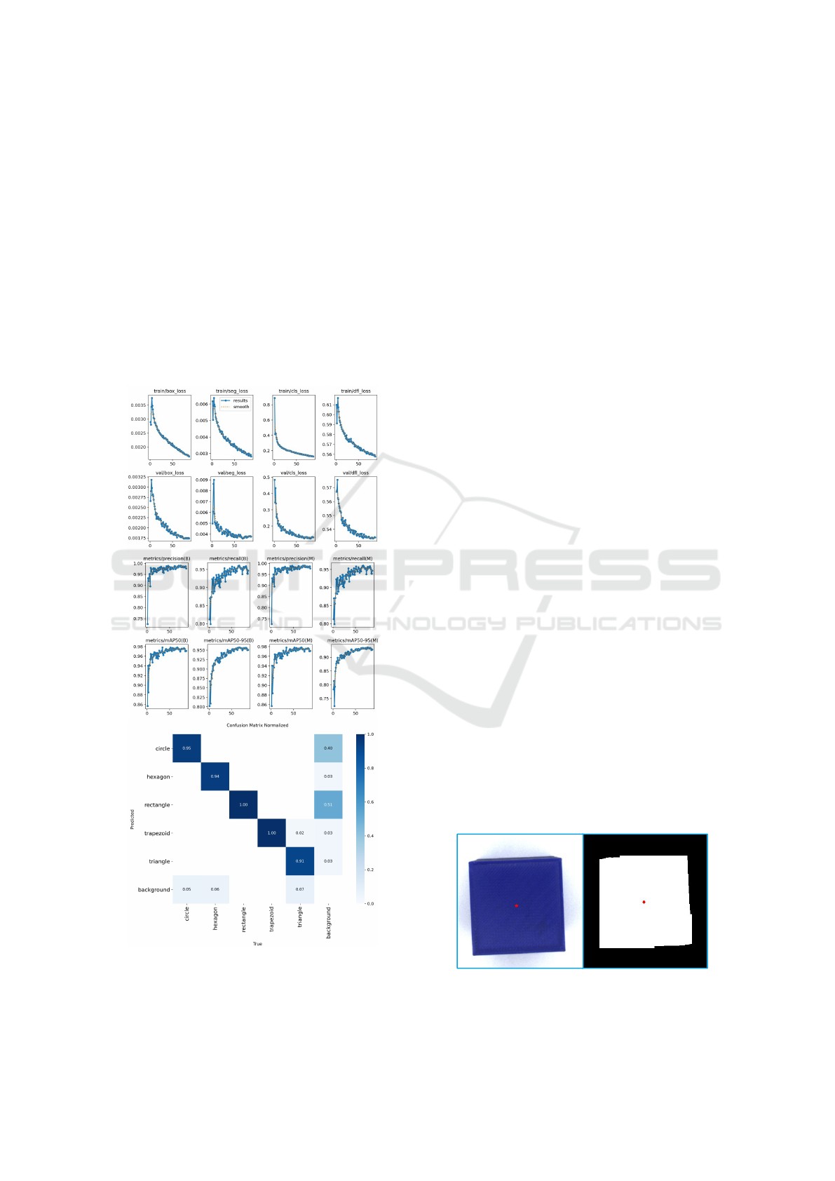
culation of the center point, which was implemented

here simply by calculating the center of gravity. Since

no center points are marked on the real objects and

printed shapes, there is no ground truth with which

the calculated center points can be compared, and so

no accuracy consideration was made here. The deter-

mination of the center points is therefore included as

an unknown in the subsequent accuracy analysis for

the triangulation.

To record data for the evaluation, the robot with

camera was moved centrally over an object placed on

the work surface. Starting from this position, a pro-

gram then always determines 51 random points within

a certain radius of the starting position. When gen-

erating the points, it is ensured that two consecutive

Figure 6: top: Graphs of the training results of the seg-

mentation model. The various loss curves, recall curves,

precision curves, and mAP values are displayed., bottom:

Confusion Matrix for the 5 different geometric shapes.

points always have a certain distance between them.

The points are then followed one after the other and

an image is taken at each position. At each position,

the camera’s viewing axis is additionally tilted by a

random angle between 5-15° towards the start posi-

tion. With our combination of working distance and

camera angle of view, this reduces the probability that

the object to be detected falls out of the camera’s ﬁeld

of view.

A stereo image pair is then always made from two

consecutive images and the center points are triangu-

lated. The triangulation always results in two posi-

tions, each based on the different viewing angles. If

these positions are close to each other, this is a charac-

teristic for a precise determination of the center point

coordinates. However, initial tests revealed signiﬁ-

cant variation in triangulation error. While an abso-

lute error of less than 1 mm was often achieved, tri-

angulations with errors of more than 10 and 20 mm

were not uncommon. For this reason, pure triangula-

tion was expanded to include mid point calculations.

First, the location of the shortest distance between

the two straight lines passing through the triangulated

point from the respective camera coordinate system

is calculated. Then, the mid point of this shortest

distance serves as the new triangulation result. The

values were compared with the center point determi-

nation based on the camera’s intrinsic and extrinsic

parameters. This method only works on surfaces cal-

ibrated to the camera or robot respectively and when

the height of the observed objects is known. Previous

work achieved accuracies ranging from 0.8 to 1.5 mm

for the x and y coordinates, depending on the working

distance.

The accuracies for squares, triangles, circles and

hexagons were evaluated. Each of the four shapes

was placed in 5 different and random positions on

the work surface, which can be seen in Figure 4.

This means that 250 triangulations were calculated for

each shape, resulting in a total of 1000 measurements.

For each random position and shape, the mean values

of the total error and its standard deviation regarding

the 2D method, mentioned before, were then deter-

Figure 7: left: image of a cube, right: segmentation mask

of the square surface of the cube.

ICINCO 2025 - 22nd International Conference on Informatics in Control, Automation and Robotics

240

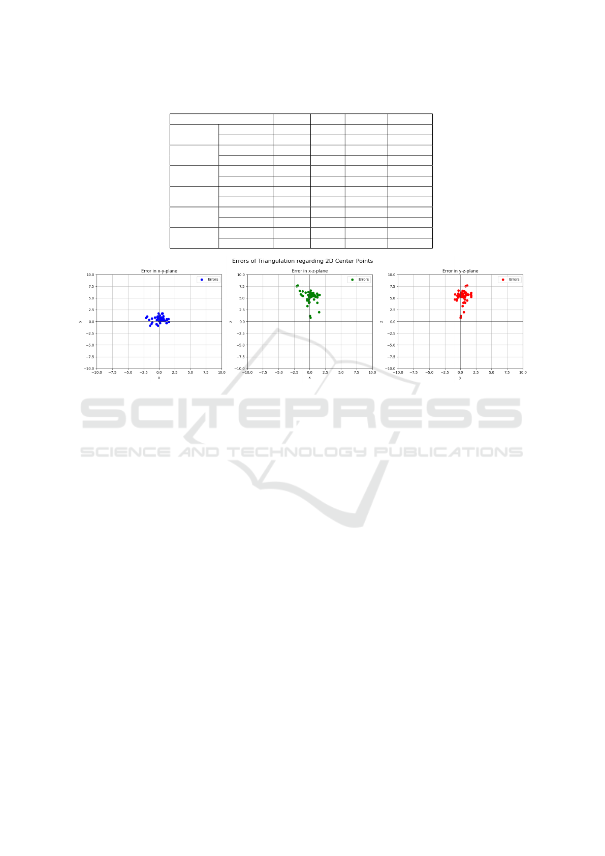
Table 1: Results of the accuracy analysis (all values in mm).

Square Circle Triangle Hexagon

Position 1

Mean Error 0.661 1.009 2.830 5.396

Std Dev 0.633 0.773 0.883 1.304

Position 2

Mean Error 1.879 1.367 2.875 6.202

Std Dev 2.629 1.392 0.917 0.492

Position 3

Mean Error 2.175 2.183 5.177 6.737

Std Dev 0.915 0.804 0.723 1.139

Position 4

Mean Error 2.837 2.931 6.147 5.984

Std Dev 0.840 0.687 1.108 0.809

Position 5

Mean Error 4.995 5.118 7.670 7.774

Std Dev 0.908 0.752 0.920 1.130

Overall

Mean Error 2.509 2.522 4.940 6.419

Std Dev 1.185 0.882 0.910 0.975

Figure 8: Triangulation error compared to the 2D method for the hexagon at position 1.

mined. The mean values of the mean values and stan-

dard deviations were then computed for each shape

and the mean values across all shapes were calculated.

The results are summarized in Table 1.

An average accuracy of 4.097 mm with a stan-

dard deviation of 0.988 mm was achieved across all

the shapes considered. The accuracy for triangles and

hexagons was particularly poor at 4.94 and 6.419 mm,

whereas circles and rectangles were located much

more accurately at 2.509 and 2.522 mm. The stan-

dard deviation, on the other hand, was fairly constant

across all four forms. Examining the composition

of the resulting error shows that the large deviations

are primarily due to differences in the Z coordinates.

Therefore, considering only the x and y coordinates

results in an average error of 0.713 mm, with a stan-

dard deviation of 0.47 mm. In comparison, the av-

erage error in the Z coordinates is 3.873 mm, with

a standard deviation of 1.102 mm. Figure Figure 8

illustrates this phenomenon by showing the triangu-

lation error compared to the 2D method for 50 mea-

surements at position 1 for the hexagon. To determine

the correct Z value, the table surface was approached

again using a TCP measured on the robot. This mea-

surement yielded a table height of -22.5 mm relative

to the robot base coordinate system. The triangulation

yielded an average table height of -21.94 mm, signif-

icantly closer to the -22.5 mm value than the -26.97

mm value determined by the 2D method.

5 CONCLUSION AND FUTURE

WORKS

In this paper, a method was presented which, based

on the recognition of simple geometric shapes, should

enable the universal identiﬁcation of matching join-

ing parts in the future. For this purpose, AI object

segmentation is combined with simple mathematical

algorithms to identify matching features. The advan-

tage of this recognition process is that new compo-

nent geometries do not have to be integrated or trained

into the object recognition process repeatedly. The

process is able to match as yet unknown objects to

each other if the cross-sections to be joined contain

simple geometric shapes such as circles, rectangles

or triangles and is therefore particularly suitable for

multi-variant productions. This method only works if

the objects to be joined do not move in space, and if

at least three geometric shapes can be recognised on

them.

An accuracy analysis was carried out for the in-

cluded AI object recognition with a YOLO model and

the subsequent stereoscopy, as this is essential to en-

able precise joining afterwards. The individual geo-

Towards Universal Detection and Localization of Mating Parts in Robotics

241

metric shapes could be triangulated with an accuracy

of less than 1 mm in some cases. The average error

was 4.097 mm, but this was due to the poor depth

values or z-coordinates of our comparison method.

When only considering errors in the x-y plane, the

average is just 0.713 mm. In principle, these results

allow the assessment that the method described here

achieves the accuracies required for a joining process,

especially if deviations occurring during joining are

also to be compensated for by force control.

In the next steps, the functionality of the method,

which was initially demonstrated on constructed ex-

amples, will also be checked on real feature sets con-

sisting of individual geometric objects and then also

tested on real components, such as connectors. As al-

ready described in Section 3, suitable tolerance win-

dows for the similarity check must then be deter-

mined.

ACKNOWLEDGEMENTS

The work presented was carried out as part of the

VADER

research project supported by the Federal

Ministry for Economic Affairs and Climate Action on

the basis of a decision of the German Bundestag and

funded by the European Union, in cooperation with

the RICAIP project

funded by European Union’s

Horizon 2020 research and innovation programme

under grant agreement No 857306.

REFERENCES

Haugaard, R. L. and Buch, A. G. (6/18/2022 - 6/24/2022).

Surfemb: Dense and continuous correspondence dis-

tributions for object pose estimation with learnt sur-

face embeddings. In 2022 IEEE/CVF Conference on

Computer Vision and Pattern Recognition (CVPR),

pages 6739–6748. IEEE.

Hodan, T., Barath, D., and Matas, J. (2020). Epos: Esti-

mating 6d pose of objects with symmetries. In 2020

IEEE/CVF Conference on Computer Vision and Pat-

tern Recognition (CVPR), pages 11700–11709. IEEE.

Irshad, M. Z., Kollar, T., Laskey, M., Stone, K., and Kira,

Z. (5/23/2022 - 5/27/2022). Centersnap: Single-

shot multi-object 3d shape reconstruction and cate-

gorical 6d pose and size estimation. In 2022 In-

ternational Conference on Robotics and Automation

(ICRA), pages 10632–10640. IEEE.

Vernetzter digitaler Assistent f

ur das datengetriebene

Engineering von roboterbasierten Produktionsanlagen

Research and Innovation Centre on Advanced Indus-

trial Production

Kuo, C.-W., Ashmore, J. D., Huggins, D., and Kira, Z.

(2019). Data-efﬁcient graph embedding learning for

pcb component detection. In 2019 IEEE Winter Con-

ference on Applications of Computer Vision (WACV),

pages 551–560. IEEE.

Liu, C., He, L., Xiong, G., Cao, Z., and Li, Z. (4/29/2019

- 5/2/2019). Fs-net: A ﬂow sequence network for

encrypted trafﬁc classiﬁcation. In IEEE INFOCOM

2019 - IEEE Conference on Computer Communica-

tions, pages 1171–1179. IEEE.

Marx, S., Gusenburger, D., Bashir, A., and M

uller, R.

(2024). Low-cost stereo vision: A single-camera ap-

proach for precise robotic perception. In Yi, J., editor,

2024 IEEE 20th International Conference on Automa-

tion Science and Engineering (CASE), pages 890–

896, Piscataway, NJ. IEEE.

Peng, S., Liu, Y., Huang, Q., Zhou, X., and Bao, H. (2019).

Pvnet: Pixel-wise voting network for 6dof pose esti-

mation. In 2019 IEEE/CVF Conference on Computer

Vision and Pattern Recognition (CVPR), pages 4556–

4565. IEEE.

Su, Y., Saleh, M., Fetzer, T., Rambach, J., Navab,

N., Busam, B., Stricker, D., and Tombari, F.

(2022). Zebrapose: Coarse to ﬁne surface encod-

ing for 6dof object pose estimation. arXiv preprint

arXiv:2203.09418.

Tekin, B., Sinha, S. N., and Fua, P. (6/18/2018 - 6/23/2018).

Real-time seamless single shot 6d object pose predic-

tion. In 2018 IEEE/CVF Conference on Computer Vi-

sion and Pattern Recognition, pages 292–301. IEEE.

Wada, K., Sucar, E., James, S., Lenton, D., and Davison,

A. J. (2020). Morefusion: Multi-object reasoning for

6d pose estimation from volumetric fusion. In 2020

IEEE/CVF Conference on Computer Vision and Pat-

tern Recognition (CVPR), pages 14528–14537. IEEE.

Wang, C., Xu, D., Zhu, Y., Martin-Martin, R., Lu, C., Fei-

Fei, L., and Savarese, S. (2019a). Densefusion: 6d ob-

ject pose estimation by iterative dense fusion. In 2019

IEEE/CVF Conference on Computer Vision and Pat-

tern Recognition (CVPR), pages 3338–3347. IEEE.

Wang, H. and Johansson, B. (8/26/2023 - 8/30/2023). Deep

learning-based connector detection for robotized as-

sembly of automotive wire harnesses. In 2023 IEEE

19th International Conference on Automation Science

and Engineering (CASE), pages 1–8. IEEE.

Wang, H., Sridhar, S., Huang, J., Valentin, J., Song, S., and

Guibas, L. J. (2019b). Normalized object coordinate

space for category-level 6d object pose and size esti-

mation. In 2019 IEEE/CVF Conference on Computer

Vision and Pattern Recognition (CVPR), pages 2637–

2646. IEEE.

Xiang, Y., Schmidt, T., Narayanan, V., and Fox, D. (2017).

Posecnn: A convolutional neural network for 6d ob-

ject pose estimation in cluttered scenes. arXiv preprint

arXiv:1711.00199.

Zakka, K., Zeng, A., Lee, J., and Song, S. (5/31/2020 -

8/31/2020). Form2ﬁt: Learning shape priors for gen-

eralizable assembly from disassembly. In 2020 IEEE

International Conference on Robotics and Automation

(ICRA), pages 9404–9410. IEEE.

ICINCO 2025 - 22nd International Conference on Informatics in Control, Automation and Robotics

242