Manipulation of Deformable Linear Objects Using Model Predictive Path

Integral Control with Bidirectional Long Short-Term Memory Learning

Lukas Zeh

, Johannes Meiwaldt, Zexu Zhou

, Armin Lechler

and Alexander Verl

Institute for Control Engineering of Machine Tools and Manufacturing Units, University of Stuttgart, Stuttgart, Germany

Keywords:

DLO, MPPI, biLSTM, Manipulation, Control, Robotics.

Abstract:

The manipulation of Deformable Linear Objects (DLOs) such as cables poses a signiﬁcant challenge for

automation due to their inﬁnite degrees of freedom and non-linear dynamics. In this paper we present a

machine learning based optimal control approach for the manipulation of DLOs. This approach is divided

into two main components: modeling and control. For modeling the dynamics of the DLO, we propose a

learning based approach using a bidirectional Long Short-Term Memory (biLSTM) network. The biLSTM

network is trained on synthetic data generated by the MuJoCo physics engine. For manipulating the DLO, a

model predictive control strategy that employs Model Predictive Path Integral (MPPI) control is selected. The

proposed approach is evaluated through simulation and experiments. The results demonstrate the effectiveness

of the proposed method in achieving accurate and efﬁcient manipulation of DLOs.

1 INTRODUCTION

Flexible objects such as textiles, cables or ropes (Mat-

suno et al., 2006) can be found almost everywhere,

both in everyday life and in the production environ-

ment. They belong to the class of deformable objects

(Keipour et al., 2022). A sub-category of deformable

objects are Deformable Linear Objects (DLOs). Ex-

amples of DLOs include cables, ropes and hoses. In

the context of robotic applications, rigid bodies are

typically assumed when gripping and manipulating

objects. This assumption is valid as long as the de-

formation of the objects is negligible. However, when

handling DLOs, the deformation of the object must be

taken into account. The automated handling of ﬂex-

ible objects by robots is a research problem that has

not yet been entirely solved (Zhu et al., 2022; Zhou

et al., 2020).

The fundamental challenge in the manipulation of

ﬂexible objects, such as DLOs, is that an external

force causes both a movement and a change in shape.

Due to the inﬁnite degrees of freedom of DLOs, mod-

eling these nonlinearities during deformation is com-

plex. Especially for real-time robotic manipulation

https://orcid.org/0000-0003-2730-1383

https://orcid.org/0009-0002-2163-2528

https://orcid.org/0000-0002-4073-1487

https://orcid.org/0000-0002-2548-6620

tasks, accurate and computationally efﬁcient dynamic

models are required. While both physics-based and

data-driven approaches exist, each has its own advan-

tages and disadvantages (Arriola-Rios et al., 2020).

To enable effective manipulation of DLOs, Model

Predictive Control (MPC) has been successfully em-

ployed for planning and control in dynamic environ-

ments involving DLOs (Yan et al., 2020; Wang et al.,

2022). MPC uses a predictive model to simulate and

optimize control actions over a ﬁnite time horizon,

making it suitable for systems with complex, time-

varying dynamics. In the context of DLOs, where

deformation must be anticipated and accounted for

during manipulation, MPC can utilise a learned or

physics-based model to generate feasible, optimized

trajectories.

This publication investigates the potential of

Model Predictive Path Integral (MPPI) control, a sam-

pling based variant of MPC, for the manipulation of

DLOs. Simulation data is generated to train the bidi-

rectional Long Short-Term Memory biLSTM network

to learn a model of the DLO dynamics ofﬂine. The

model is then used in an MPPI controller to determine

the trajectories for manipulating the DLO.

The contribution of our work can be summarized

as follows:

• We contribute datasets, model architecture and

model weights for modeling cables. The datasets,

model architecture and model weights are avail-

Zeh, L., Meiwaldt, J., Zhou, Z., Lechler, A. and Verl, A.

Manipulation of Deformable Linear Objects Using Model Predictive Path Integral Control with Bidirectional Long Short-Term Memory Learning.

DOI: 10.5220/0013703800003982

Paper published under CC license (CC BY-NC-ND 4.0)

In Proceedings of the 22nd International Conference on Informatics in Control, Automation and Robotics (ICINCO 2025) - Volume 1, pages 47-58

ISBN: 978-989-758-770-2; ISSN: 2184-2809

able at https://doi.org/10.18419/DARUS-5050.

• We propose a framework for the manipulation of

DLOs that utilizes a Model Predictive Path Inte-

gral Controller to manipulate deformable objects.

• We demonstrate the effectiveness of our proposed

method in simulation and experiments.

The paper is organised as follows: In Section II, we

review related work. The dataset is introduced in Sec-

tion III, and our proposed framework is established in

Section IV. In Section V, we present our simulation

and experimental results.

2 RELATED WORK

The precise manipulation of Deformable Linear Ob-

jects (DLOs) requires a physics-based model that ac-

counts for both deformation and an appropriate rep-

resentation of object shape (Sanchez et al., 2018).

Modeling approaches can generally be divided into

physics-based and data-driven methods (Arriola-Rios

et al., 2020).

2.1 Physics-Based Modeling

Approaches

There are various physics-based modeling approaches

for DLOs. Particle-based models describe DLOs

as discrete particles whose positions change in ac-

cordance with Newton’s laws under the inﬂuence of

forces. In mass-spring-damper systems, these parti-

cles are connected by springs, and their physical pa-

rameters are described using parameters such as stiff-

ness and damping (Schulman et al., 2013). Although

these models are computationally efﬁcient, they re-

quire precise parameterization, which limits their ap-

plicability to real-world industrial cables (Monguzzi

et al., 2025).

Point-based dynamics (PBD), on the other hand,

use geometric constraints to directly compute parti-

cle positions. They are more memory- and compute-

efﬁcient than mass-spring systems but less physically

accurate (Arriola-Rios et al., 2020).

To achieve a more physically accurate represen-

tation, the DLO is discretized using Finite Element

Methods (FEM) and the deformation equations are

solved through numerical integration. However, FEM

approaches are computationally intensive and require

accurate material parameters (Koessler et al., 2021;

Yin et al., 2021). As a result, they are generally un-

suitable for real-time robotic manipulation tasks un-

less speciﬁc simpliﬁcations are made.

Other numerical methods make assumptions, such

as the absence of large deformations, which limits

their applicability in more dynamic tasks (Rabaetje,

2003). Meanwhile, Jacobian-based approaches use

local approximations to relate the movement of the

robot to the deformation of the object. While these

approaches are real-time capable, they only compute

local deformation models (Zhu et al., 2022).

2.2 Data-Driven Approaches

Data-driven models have gained popularity due to

their ability to capture the complex nonlinear dynam-

ics of DLOs. These models are trained using either

simulated (ofﬂine) data or real-world (online) data.

When using simulated data, physical-based models

are typically employed to generate the training data.

The advantage of using simulated data is the ease and

speed of data generation compared to collecting real-

world data.

Several deep learning approaches have been pro-

posed. For example, bidirectional Long Short-Term

Memory (biLSTM) networks have been used to prop-

agate DLO dynamics over time (Yan et al., 2020;

Yang et al., 2022). The interaction-biLSTM pro-

posed by Yang et al. outperformed a baseline biLSTM

model in terms of accuracy, although with slightly re-

duced computational efﬁciency.

Graph Neural Networks (GNNs) have also been

adopted to model DLO dynamics (Wang et al., 2022;

Cao et al., 2024). In GNN-based methods, the DLO

is represented as a graph of discrete capsule elements

connected by physically motivated constraints such as

bending stiffness, length restrictions, and collisions.

The nodes represent DLO elements, and the edges

capture the interactions between them.

Another approach uses radial basis function net-

works to estimate local deformation models via Ja-

cobian matrices, encoding the relationship between

DLO deformation and the robot end-effector position

(Yu et al., 2023).

While these methods are capable of modeling the

complex dynamics of DLOs, they typically require

large datasets to achieve robust performance. It is

therefore essential to assess whether models trained

on simulation data generalize well enough for real-

world robotic manipulation.

2.3 Model Predictive Control for DLO

Manipulation

Model Predictive Control (MPC) is a strategy used

for manipulating DLOs (Wang et al., 2022). It relies

on predictive models to simulate object dynamics and

ICINCO 2025 - 22nd International Conference on Informatics in Control, Automation and Robotics

optimize control actions over a time horizon. The pre-

dictive model can be either physics-based or learned

from data. MPC is particularly effective for ma-

nipulating deformable objects as it enables forward-

looking planning that takes into account the evolution

of the object’s shape.

A sampling-based variant of MPC, Model Predic-

tive Path Integral (MPPI) control, was ﬁrst introduced

in (Williams et al., 2016) for the autonomous driving

of a high-speed RC car. In (Williams et al., 2017),

the authors generalized and formalized the MPPI

approach, proposing a learning-based, information-

theoretically grounded formulation. This extension

makes MPPI applicable in data-driven and model-

uncertain scenarios. Since then, MPPI has been ap-

plied in various robotic domains (Yan et al., 2020;

Bhardwaj et al., 2021; Pezzato et al., 2025). The

STORM framework, introduced in (Bhardwaj et al.,

2021) is a fast, sampling based model predictive con-

trol framework that works directly in joint space.

It enables real-time responses to complex manipula-

tion tasks, including collisions, joint boundaries and

uncertain perception, through GPU parallelization.

(Pezzato et al., 2025) use a GPU-based physics sim-

ulator as the dynamic model for MPPI control. This

allows high-contact tasks to be solved without explicit

modeling or learning, offering a fast, ﬂexible and ro-

bust solution in the presence of uncertainties. (Yan

et al., 2020) used MPPI control to show the effec-

tiveness of their Coarse-to-ﬁne rope state estimation

method. In their work the MPPI controller is used

to estimate the optimal gripping point of the rope for

manipulating the rope into a desired shape.

We extend existing works by applying MPPI con-

trol to manipulate different types of DLOs. We chose

a biLSTM model for modeling the DLO dynamics

based on the combination of high inference speed, ac-

ceptable accuracy and suitability for robust, ﬂexible

control. To ensure optimal performance, we conduct

a hyperparameter search to identify the best model

conﬁguration. The biLSTM model is used in com-

bination with a MPPI controller to generate optimal

trajectories for DLO manipulation. The effectiveness

of our approach is demonstrated through simulation

and experimental results.

3 DATASET

In the following, we describe the dataset used to train

the biLSTM model.

3.1 Simulation Environment

The datasets used to train the biLSTM model were

generated using the MuJoCo (Todorov et al., 2012)

physics engine. MuJoCo natively provides a plugin

for the simulation of DLOs. In this plugin, DLOs are

approximated as mass-spring systems. The DLO is

modeled as a chain of mass points, which are con-

nected by linear, torsional, and bending springs. The

individual spring-mass elements are modeled in sim-

pliﬁed manner as capsules with the corresponding

physical properties. This approach saves time in the

modeling process and also allows for a simple and in-

tuitive implementation. Furthermore, it has the ad-

vantage that the parameters of the DLO can be eas-

ily and quickly adjusted, enabling a wide range of

DLO variations to be simulated. To train the biLSTM

model, a DLO with a length of 0.5 m was modeled

in MuJoCo, consisting of 50 capsules with a diam-

eter of 1 cm. The number of 50 capsules was cho-

sen as a compromise between realistic behavior and

computation time. The higher the number of cap-

sules, the more degrees of freedom the system has.

This increase in degrees of freedom leads to an almost

exponential increase in computation time required to

simulate the DLO. The parameters to be set in the

simulation are the Young’s modulus [Pa], the shear

modulus [Pa], and the damping [Nms/rad] between

the individual capsules. Young’s modulus was cho-

sen as 4 × 10

Pa, the Shear modulus as 1 × 10

Pa,

and the damping was set to 1 Nms/rad. For the train-

ing of the biLSTM model, a simulation step time of

1 ms was chosen. The individuzal trajectories within

the datasets have a length of 5 s. Inﬂuences of grav-

ity, friction, and air drag are not considered in the

simulation. Figure 1 shows the data generation pro-

cess. For the simulation, the DLO is ﬁxed at the right

end with a welding condition, so that this end be-

haves like a clamped end. The left end of the DLO

is manipulated by a robot arm. The robot arm per-

forms a random trajectory in the xy-plane at a height

of 0.15 m. For the data generation, the cable is ma-

nipulated from a straight line into a random shape by

moving the left end of the DLO to a random posi-

tion within the green box. The target position of the

robot is chosen randomly for each trajectory within

the range of x ∈ [0.05, 0.35] m and y ∈ [−0.2, 0.2] m

(green area in Figure 1). The origin coordinate sys-

tem is located in the center of the manipulated cap-

sule. To generate a wider range of deformations, the

DLO is also randomly rotated around the z-axis in the

range of ψ ∈ [−1, 1] rad. The target position range

was chosen to avoid overstretching the DLO. During

the data generation, the positions of the 50 capsules

Manipulation of Deformable Linear Objects Using Model Predictive Path Integral Control with Bidirectional Long Short-Term Memory

Learning

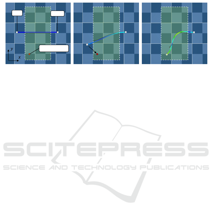
target position

fixed

free

Figure 1: Dataset Generation. The cable is manipulated from a straight line to a random shape by moving the free end of the

cable to a random position within the green box.

DLO

, the end effector position X

TCP

, and velocity

TCP

are recorded.

3.2 Representation of DLO in 2D

Since the manipulation takes place on a surface, we

chose a representation of the DLO in 2D, similar to

(Yan et al., 2020). For the training of the biLSTM

model, the simulation data is reduced. Instead of us-

ing all 50 simulated capsules, in order to reduce the

computing time, only every 5th capsule is used for

training, resulting in a total of n = 10 capsules. The

ﬁrst and last capsules are also removed, as these are

not needed for predicting the DLO dynamics. The

position of the ﬁrst capsule is described by the pose

of the end effector X

TCP

. The position of the last

capsule remains constant due to the welding con-

dition. The position of the DLO can therefore be

described as a sequence of points in 3D Cartesian

space X

DLO

∈ R

n×2

. For better generalization of

the biLSTM model, the relative position of the cap-

sules with respect to the end effector position x

TCP

is used instead of the absolute position, computed as

r,i

= x

− x

TCP

for i = 1, . . . , n. For the calculation of

the relative positions, only the x and y coordinates are

used, as the z-coordinate is constant due to the ﬁxed

height of the end effector. The relative positions of

the individual capsules of the DLO are described by

DLO

= (x

r,1

, x

r,2

, ..., x

r,n

). (1)

The advantage of this representation is the transla-

tional invariance, which allows the neural network to

learn the deformation of the DLO not from the ab-

solute positions, but by directly linking the deforma-

tion to the end effector position. The velocity of the

capsules is described by the difference of the relative

positions at time t and t − 1. The overall state of the

DLOs is described by

DLO

= (X

DLO

). (2)

The state of the end effector is described by the Carte-

sian position of the end effector, as well as the rotation

of the end effector around the z-axis. The state of the

end effector is therefore described in detail as follows:

TCP

= (X

TCP

) = ((x, y, z, ψ), ( ˙x, ˙y, ˙z,

ψ)). (3)

The overall state of the system

= (S

DLO

, S

TCP

), (4)

is obtained by combining the state of the DLO and the

state of the end effector.

4 PROPOSED FRAMEWORK

In this section, we introduce the proposed framework

for cable manipulation. The manipulation of the cable

is done in 2D. First, an overview of the system used

for the manipulation task is given. Then, the bidirec-

tional Long-Short-Term-Memory (biLSTM) model

for modeling the DLO dynamics is introduced. Fi-

nally, the Model Predictive Path Integral (MPPI) con-

troller used to manipulate the DLO to the desired

shape is described.

4.1 System Overview

The framework for cable manipulation, as displayed

in Figure 2, consists of a biLSTM model and a MPPI

controller. As an input for the system, the current state

of the DLO S

g,t

and the desired shape of the DLO

tar

are used. The current state of the DLO, S

DLO

, is

deﬁned by the relative positions and velocities of the

capsules, as described in the previous section. The

desired shape of the DLO is represented by the target

position of the capsules. Based on the current state of

the DLO and the desired shape, the MPPI controller

generates a set of random trajectories U

. These tra-

jectories are then sent to the biLSTM model, which

ICINCO 2025 - 22nd International Conference on Informatics in Control, Automation and Robotics

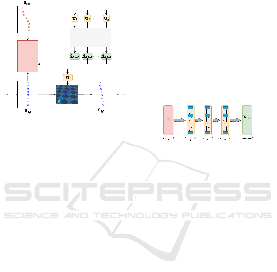
robot TCP

MPPI

controller

biLSTM

model

Figure 2: The proposed framework for cable manipulation

uses a biLSTM model trained on synthetic data to predict

DLO deformation. This prediction is passed to the MPPI

controller, which computes the optimal robot control input.

predicts the velocities of the capsules for the next time

step

. The information about the resulting defor-

mation of the DLO is then used to calculate the cost

function for the MPPI controller. The best trajectory

is selected based on the cost function and sent to the

robot for execution. This execution leads to a new

state of the DLO S

g,t+1

, which is then used as input

for the next iteration of the MPPI controller. The pro-

cess is repeated until the DLO has reached the desired

shape.

4.2 biLSTM Cable Model

As in the works of (Yang et al., 2022), (Yan et al.,

2020), and (Gu et al., 2025), a biLSTM model is em-

ployed for modeling the DLO, as it has been shown

to effectively capture its dynamic behavior. The

biLSTM model is a type of recurrent neural net-

work (RNN) that is particularly well-suited to se-

quence prediction tasks. The biLSTM is able to cap-

ture the dynamics and temporal dependencies of the

DLO by processing the sequence of relative positions

of the capsules and their velocities. Unlike standard

RNNs, information ﬂows in both temporal directions,

allowing the model to use both past and future con-

text for improved sequence understanding. This fea-

ture allows for more effective modeling of relation-

ships along the DLO structure. This bidirectional

processing enhances the LSTM’s ability to capture

long-range interactions, improving its performance in

sequential deformation modeling tasks. Compared

to unidirectional networks such as MLPs, standard

RNNs, or unidirectional LSTMs, biLSTMs have ad-

vantages in modeling the complex dynamics of de-

formable linear objects (Yang et al., 2022). To bet-

ter capture the coupled dynamics, the biLSTM addi-

tionally incorporates the end-effector state as input,

enabling the model to learn the interaction between

actuator motion and DLO deformation. Thus, the

complete system state S

is provided as input to the

biLSTM model. The general structure of the biLSTM

model is shown in Figure 3. Its architecture consists

of an input layer, one or more stacked biLSTM layers,

and a fully connected output layer. This output layer

predicts the capsule velocities for the next time step.

The predicted velocities are then used to compute the

cost function for the MPPI controller.

Input

1. biLSTM

layer

Output

2. biLSTM

layer

3. biLSTM

layer

Figure 3: The biLSTM architecture used for modeling the

DLO consists of an input layer, three biLSTM layers and an

output layer.

4.2.1 Training

The biLSTM model is trained on the data generated

in the simulation environment. The biLSTM model

is trained using 10,000 trajectories. These trajectories

are split into training and test data, with 80 % of the

data used for training and 20 % for testing. The train-

ing is performed using the Adam optimizer and the

Mean Squared Error (MSE) loss function. The MSE

loss function is deﬁned as:

MSE(y, ˆy) =

∑

i=1

−

)

, (5)

where N is the number of nodes, y

is the true veloc-

ity of the node i and

is the predicted velocity of the

node i. To determine the optimal hyperparameters for

the biLSTM model, both a random search and a grid

search were performed. The random search was used

to perform an initial narrowing down of the hyperpa-

rameters. The random search showed that the most

effective models consistently used a hidden layer size

of 256 or 512, were trained for up to 100 epochs, and

employed a learning rate between 1e-5 and 1e-3. A

low weight decay between 1e-7 and 1e-5 was also

common among top-performing conﬁgurations. The

number of biLSTM layers varied between 2 and 6, in-

dicating that model depth was less critical compared

to other parameters. Training the model for more

than 50 epochs didn’t yield signiﬁcant improvements,

Manipulation of Deformable Linear Objects Using Model Predictive Path Integral Control with Bidirectional Long Short-Term Memory

Learning

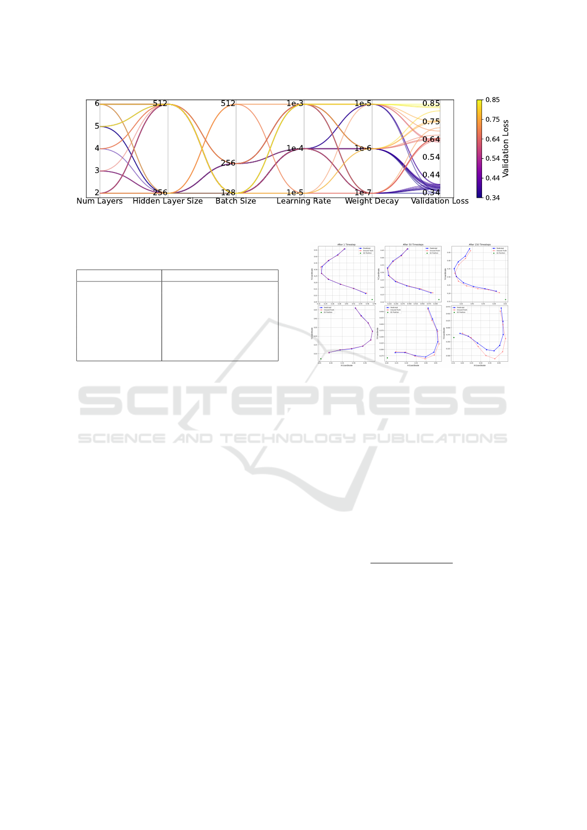
Figure 4: Performance of the biLSTM model in terms of validation loss for different hyperparameter combinations. Visualized

are the top 10 % and the bottom 10 % of hyperparameter combinations during grid search.

Table 1: Hyperparameters of the biLSTM model, bold val-

ues are also used for grid search.

Hyperparameter Values Random Search

biLSTM Layers [1, 2, 3, 4, 5, 6]

Hidden Layer Size [8, 16, 32, 64, 128, 256,

512, 1024]

Epochs [10, 20, 30, 40, 50, 100]

Batch Size [16, 32, 64, 128, 256, 512]

Learning Rate [1e-3, 1e-4, 1e-5, 1e-6]

Weight Decay [1e-4, 1e-5, 1e-6, 1e-7]

suggesting that the model converged well within this

range. In contrast, poor performance was associated

with smaller hidden layer sizes, overly small learning

rates, high weight decay values, and very small batch

sizes. These results suggest that model capacity, suf-

ﬁcient training duration, and a well-tuned optimiza-

tion setup are essential for achieving high prediction

accuracy. Based on these ﬁndings, a subsequent grid

search was then used to ﬁnd the optimal hyperparame-

ters in a smaller range. In the table 1, the hyperparam-

eters of the biLSTM model are summarized. Figure

4 shows the model performance of various hyperpa-

rameter combinations, obtained through grid search,

in terms of the validation loss.

Based on the hyperparameter study, the model

with the best performance in terms of validation loss

was selected. The model was trained using a learning

rate of 1e-4 in combination with a weight decay of 1e-

7. The model with the best performance was trained

with batchsize 128 and consists of three biLSTM lay-

ers, as shown in Figure 3. Each biLSTM layer con-

sists of 512 neurons (this is equivalent to a hidden

layer size of 256 neurons in each direction). In the

following section, the performance of this model is

evaluated.

4.2.2 Model Evaluation

In order to use the biLSTM model in simulation or

Model Predictive Control (MPC), a precise rollout

prediction over multiple time steps is crucial. A roll-

Figure 5: Shape-error e

shape,biLSTM

after 1, 50 and 150

timesteps. The blue line represents the model prediction,

while the transparent red line represents the ground truth.

out is a sequence of predicted states over a certain

time horizon, which is used to evaluate the model’s

performance in predicting the DLO dynamics. The

quality of the dynamic model signiﬁcantly inﬂuences

the selection of optimal control sequences. The model

quality is evaluated based on rollouts over 50 time

steps (equivalent to 1 second) and 150 time steps

(equivalent to 3 seconds). As a metric for the model

quality, the average shape error e

shape

and the average

velocity error e

vel

are used.

shape, biLSTM

= ∥x

groundtruth

− x

pred

∥

, (6)

vel, biLSTM

∥

groundtruth

−

pred

∥

groundtruth

∥

× 100 %. (7)

The model is evaluated on 100 rollouts, each with

a length of 150 time steps (3 seconds). The average

shape error e

shape, biLSTM

and the average velocity er-

ror e

vel, biLSTM

are calculated over all rollouts. The

model is able to predict the shape of the DLO with an

average shape error e

shape, biLSTM

of 3.3 cm and the ve-

locity with an average velocity error e

shape, biLSTM

61.59 % (similar to those in (Yang et al., 2022)). The

error of both the shape and the velocity increases with

the number of time steps. Figure 5 shows qualita-

tive results of the shape error over 1, 50 and 150 time

steps. The blue line represents the model prediction,

ICINCO 2025 - 22nd International Conference on Informatics in Control, Automation and Robotics

while the transparent red line represents the ground

truth. The biLSTM model shows stable predictions,

even over long time intervals. Structure, length and

curvature are preserved, indicating a high model ca-

pacity and robust dynamic capture.

4.3 Model Predictive Path Integral for

Manipulation

Model Predictive Control (MPC) is a well-established

control strategy that has been successfully used to ma-

nipulate deformable objects (Wang et al., 2022; Yu

et al., 2022). In this paper, the DLO is manipulated

using a Model Predictive Path Integral (MPPI) based

control strategy, similar to that in (Yan et al., 2020)

and (Williams et al., 2016). MPPI is a sampling-based

Model Predictive Control strategy particularly suited

to handling complex systems and multiple objectives.

In this context, MPPI is employed to compute a

control strategy that transforms an initial conﬁgura-

tion into a desired target conﬁguration through shape

control. Actions are represented as target positions

for the end effector (EE).

The MPPI algorithm is based on the principle of

sampling multiple control sequences around a nomi-

nal sequence. A new control sequence is then gener-

ated as a weighted average of these control sequences.

This new sequence is then used to construct the nom-

inal control sequence for the next iteration.

A special feature of MPPI lies in the evaluation

of the simulated trajectories. Each trajectory is as-

signed a cost value indicating how well the system

performs under the respective control inputs. After

simulating numerous future trajectories, each trajec-

tory is assigned a unique set of disturbance values.

The MPPI algorithm calculates a weighted sum of

these disturbances. This nominal control sequence is

initialized using one of two alternative mechanisms.

When no prior solution exists, a zero-valued sequence

spanning the planning horizon is used as the starting

point. However, when a previous solution is available,

a receding horizon approach is employed. In this ap-

proach, the prior solution is propagated forward by

one timestep and the terminal control action is reset

to zero. This warm-start methodology maintains so-

lution continuity while adhering to the principles of

Model Predictive Control.

Each trajectory is evaluated based on its cost

value, with lower-cost trajectories receiving higher

weights and thus have a greater inﬂuence on the con-

trol update. Speciﬁcally, the weight of a trajectory is

determined by the exponential function of the nega-

tive ratio of its cost to a ﬁxed parameter λ, also known

as temperature (Williams et al., 2017):

= e

−

, (8)

where s

represents the cost of trajectory k. The cost

function used in MPPI consists of two terms: a shape

cost and a control cost. The shape cost penalizes de-

viations from the target conﬁguration and is deﬁned

using the Euclidean seminorm:

= 0.5 ·

∑

i=1



⊤

shape,i

· Q · e

shape,i



, (9)

where Q = diag(w

, w

, . . . , w

) is a diagonal matrix

assigning positive weights w

to each feature point in

the plane. The control cost penalizes excessive input

effort and is given by:

= 0.5 ·

∑

i=1



⊤

b,i

· R · u

b,i



, (10)

where R is the weighting matrix for the sampled con-

trol inputs u

To compute a valid probability distribution over

trajectories, the raw weights are normalized:

˜w

∑

j=1

. (11)

This normalization ensures that trajectories with

lower costs contribute more strongly, while keeping

the overall inﬂuence balanced.

The MPPI (Model Predictive Path Integral) algo-

rithm proceeds as described in Algorithm 1. It begins

with the initialization of a nominal control sequence

U = {u

, u

, . . . , u

N−1

}, which is typically initialized

to zero. In each iteration, a set of K trajectories is gen-

erated by sampling random disturbances δu

for every

time step across the prediction horizon. These distur-

bances are added to the nominal control sequence to

create perturbed control sequences. These are then

used in a Monte Carlo tree search. For generating

the random disturbances δu

, pink noise (Eberhard

et al., 2023) is used. Each control sequences simu-

lates the system’s response to the disturbed input se-

quence. For deformable linear object (DLO) manipu-

lation, this simulation is performed using the biLSTM

model, which predicts the resulting DLO states

based on the current system state S

g,t

and the sam-

pled control input. The resulting trajectory is evalu-

ated using a cost function that measures the deviation

from the target state S

tar

as well as the control effort.

The total cost of each trajectory s

is computed, and

the corresponding weight ˜w

is derived as described

above. The nominal control sequence is then updated

using a cost-weighted average of the disturbances:

U ← U +

∑

k=1

˜w

· δu

. (12)

Manipulation of Deformable Linear Objects Using Model Predictive Path Integral Control with Bidirectional Long Short-Term Memory

Learning

This update shifts the nominal inputs towards those

associated with lower-cost trajectories, thereby grad-

ually improving control performance. The updated

control input is applied to the system, which advances

by one time step. The resulting new system state is

recorded and used as input to the biLSTM model for

the next iteration. The ﬁrst element u

of the opti-

mized control vector U, produced by the MPPI con-

troller, is applied to the robot or EE. The resulting

system state is then updated. This process is repeated

until a termination condition is met, either after a

ﬁxed number of iterations or when the distance error

threshold is reached.

Data: Initial state S(g, t

), model dynamics,

cost function, prediction horizon N,

number of control sequences K

Result: Optimized control input sequence

0..N−1

initialize control sequence U

0..N−1

;

while target not reached do

generate random disturbances δU;

for control sequences k = 1..K do

start at current state X

k,0

= X(t

);

for horizon steps n = 0..N − 1 do

input U

k,n

= U

+ δU

k,n

;

next state

k,n+1

= biLSTM(X

k,n

, U

k,n

);

trajectory cost s

= control cost

+ shape cost C

;

end

for n = 0..N − 1 do

+ = reward-weighted disturbance;

end

apply ﬁrst input U

as control input;

receive current state;

check if target is reached;

end

Algorithm 1: MPPI Monte-Carlo-Algorithmus.

As shown in Figure 2, this complete process en-

ables model-based manipulation of deformable ob-

jects by optimizing a control sequence that minimizes

cost while adapting to the predicted system dynamics.

5 SIMULATION AND

EXPERIMENTS

In this section, the simulation and experimental re-

sults are presented and discussed. The goal of the sim-

ulation and experiments is to analyze the behavior of

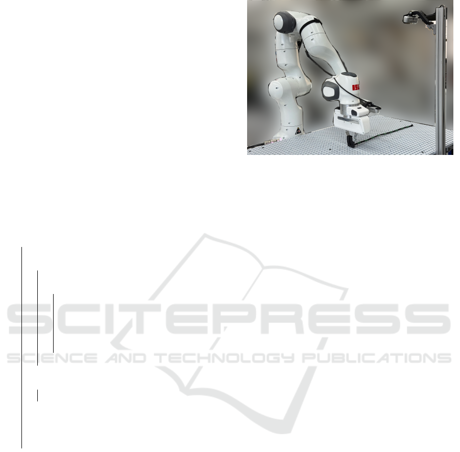
Figure 6: Experiment Setup.

the DLO and the performance of the MPPI controller.

The simulation and experiments are performed with a

Franka Emika Panda robot. First, the simulation and

experimental setup is described. Then, the results are

presented and discussed.

5.1 Simulation and Experimental Setup

1. Simulation Setup: The simulation environment

is built using the MuJoCo physics engine. As in

the simulation, the cable has a length of 50 cm

and a diameter of 1 cm. Young’s modulus is

4 × 10

Pa, the Shear modulus is 1 × 10

Pa and

damping is set to 1 Nms/rad. One Franka Emika

Panda robot moves one end of the cable so that the

shape of the cable matches the desired shape. The

other end of the cable is ﬁxed.

2. Experiment Setup: The experimental setup is

shown in Figure 6. A Franka Emika Panda robot

is used to manipulate the cable so that the shape

of the cable matches the desired shape. The other

end of the cable is ﬁxed using two zip ties. An

Intel Realsense D435i RGB-D camera is used to

track the shape of the cable. The biLSTM model

and the MPPI controller are implemented on a

Ubuntu 24.04 real-time desktop computer. The

robot trajectories are sent to the robot for execu-

tion with a communication frequency of 1,000 Hz.

The camera data is processed with 40 fps.

5.2 Simulation Results

In the following, the results of the simulation are pre-

sented. The simulation was performed using the Mu-

JoCo model of the Franka Emika Panda robot pro-

vided by the MuJoCo physics engine. The left end of

the DLO is ﬁrmly gripped by the end effector of the

robot. The right end of the DLO is ﬁxed. The initial

pose of the robot is set to reﬂect the initial position

ICINCO 2025 - 22nd International Conference on Informatics in Control, Automation and Robotics

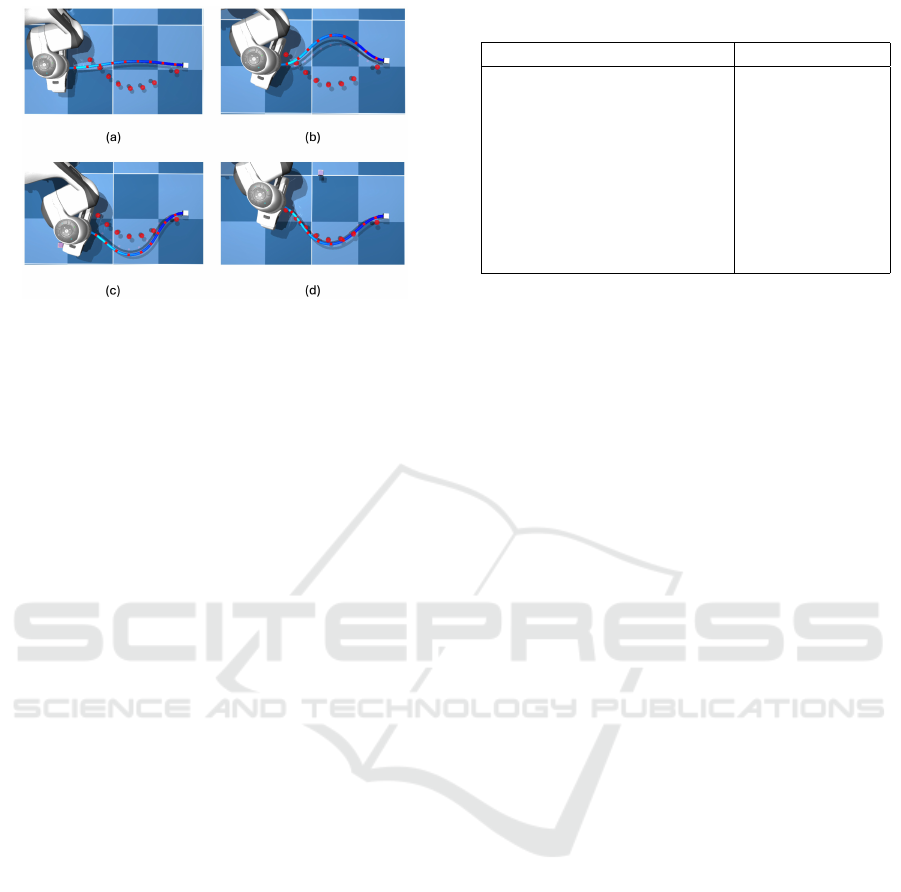
Figure 7: Steps of the shape control in the simulation envi-

ronment.

of the DLO, meaning the robot is positioned so that

the DLO is in a straight line. Each control output of

the MPPI controller is set as the target position for a

motion capture body. This body serves as the Carte-

sian target position for the inverse kinematics control

of the robot. The control process was performed in

the x-y-plane, while the z-position was kept constant

at 10 cm. The rotation around the z-axis also received

a direct control input from the MPPI output. The con-

trol values were limited to a range of -0.2 m to 0.2 m

in the x-direction and 0 m to 0.35 m in the y-direction.

This reﬂects the workspace during the generation of

the training data. The parameters of the MPPI con-

troller are displayed in Table 2. These parameters

were determined empirically through a series of ex-

periments.

First, the performance of the MPPI controller is

evaluated by shaping the DLO into a U-shape. Figure

7 shows the process of the shape control in the sim-

ulation. In (a), the initial state of the DLO is shown.

In (b), the DLO is deformed to the opposite side of

the target position. In (c), the MPPI control could

compensate for the initial deformation and move the

DLO to the other side. In (d), the MPPI control

has approached the target position and the trial has

ended. 100 trials were performed, with a success cri-

terion being a maximum deviation of 2 cm between

the positions of the simulated capsules (represented

by red dots on the cable) and their corresponding tar-

get points (represented by red dots on the plane). The

success rate was 93 %, with an average time of 7.26 s

per successful trial. A successful trial is deﬁned as

a trial in which the DLO is shaped into the desired

U-shape within 30 seconds.

Additionally, the performance of the MPPI con-

troller is evaluated over 1,000 trials of shaping the

DLO into random goal shapes. The success rate was

20.5 %, with an average time of 13.3 s per successful

Table 2: MPPI parameters in simulation.

Parameter Value

Horizon (H) 5

Time increment (dt) 0,2

Number of samples (N) 20

Temperature (λ) 0.002

Standard deviation of the

disturbances (δ)

[0.5;0.5;0; 3]

for [X, Y, Z, Rot(Z)]

Form error weighting (Q) 150

Control error weighting (R) 5

trial.

The simulation results show that the MPPI-based

control in combination with a biLSTM dynamics

model is able to shape the DLO into a desired target

shape. The approach combines sample-based control

with a neural network for modeling the DLO dynam-

ics. By training with relative positions of the capsules,

the approach can also be transferred to new scenarios.

However, re-optimizing the MPPI parameters is nec-

essary in scenarios where the target shape differs sig-

niﬁcantly from the one for which the controller was

originally tuned. Additional parameterization is also

required to handle severe deformations of the DLO

effectively. One limiting factor is the computational

demand of the biLSTM model, especially when pro-

cessing a large number of fault samples. Increasing

computing resources could improve the controller’s

performance, as a larger sample size generally leads

to greater accuracy and robustness. Another poten-

tial bottleneck is the current sampling strategy used by

the MPPI controller. Using an adaptive sampling ap-

proach where exploration during the construction of

the search tree focuses only on trajectories with high

solution potential, might improve the results.

5.3 Experiment Results

The performance of the MPPI controller is evaluated

across three different scenarios. In the ﬁrst scenario,

2D shape control is performed on a 50 cm long cable

with a diameter of 6 mm, equipped with 9 markers.

The second scenario uses the same cable and marker

setup, but shape control is conducted in 3D. The third

scenario involves 2D shape control of a 50 cm long

wire with a diameter of 1.5 mm, without any mark-

ers. While initial parameter tuning was performed in

simulation, further adjustments were necessary dur-

ing practical validation to compensate for discrepan-

cies between simulated and real-world behavior. The

MPPI controller parameters remain consistent across

all scenarios and are listed in Table 3.

In all three scenarios, the cable is manipulated into

Manipulation of Deformable Linear Objects Using Model Predictive Path Integral Control with Bidirectional Long Short-Term Memory

Learning

Table 3: MPPI parameters in experiment.

Parameter Value

Horizon (H) 8

Time increment (dt) 0.02

Number of samples (N) 200

Temperature (λ) 0.002

Standard deviation of the

disturbances (δ)

[0.2;0.2;0; 0.02]

for [X, Y, Z, Rot(Z)]

Form error weighting (Q) 150

Control error weighting (R) 5

Figure 8: Experiment result of the 2D shape control of a

50 cm long cable with a diameter of 6 mm, marked with 9

markers. The cable is manipulated into a U-shape.

a U-shape. The goal of the shape control experiments

is to shape the cable into the desired U-shape with

a maximum deviation of 2 cm from the target posi-

tion. The derivation of the target position is based

on the difference between the measured positions of

the markers on the cable and the target positions of

the markers. In the ﬁrst and second scenario, 9 mark-

ers along the cable are used to track the shape of the

cable. The positions of these markers are tracked us-

ing a color ﬁlter. In the third scenario, no markers

are used to track the shape of the cable. Instead, the

FastDLO algorithm (Caporali et al., 2022) is used for

shape estimation. Based on the estimated shape, 9

virtual markers are placed along the tracked shape in

order to keep the process of the shape control as sim-

ilar as possible to the ﬁrst two scenarios.

In the ﬁrst scenario, the cable is mounted directly

on the working plane. In Figure 8, the process of a

successful 2D shape control is shown. Indicated are

the initial state of the cable and robot (1), two inter-

mediate states (2) and (3), and the ﬁnal state of the

cable and robot (4), where the cable has been suc-

cessfully shaped into the desired U-shape. To evalu-

ate the performance of the MPPI controller, 20 trials

were performed. The success rate was 85 %, with an

average time of 15.7 s per successful trial. The fastest

trial took 2.1 s, and the slowest took 45.2 s. In the

second scenario, the cable is mounted on a 7 cm high

platform. As in the ﬁrst scenario, the 9 markers are

Figure 9: Experiment result of the 3D shape control of a

50 cm long cable with a diameter of 6 mm, marked with 9

markers. The cable is manipulated into a U-shape.

Figure 10: Experiment result of the 2D shape control of a

50 cm long wire with a diameter of 1.5 mm. The cable is

manipulated into a U-shape.

used to track the shape of the cable. The positions of

these markers are tracked by using a color ﬁlter. In

Figure 9, the process of a successful 3D shape control

is shown. The starting position of the robot remains

the same as in the ﬁrst scenario. This leads to the

cable being slightly bent by gravity at the beginning

,which can be seen in (1). In (2) and (3), two inter-

mediate states of the shape control are displayed. The

ﬁnal state of the cable and robot can be seen in (4),

where the cable has been successfully shaped into the

desired U-shape.

Even though this scenario was not trained, the

MPPI controller is able to manipulate the cable into

a U-shape. The process of the shape control is not

as roboust as in the ﬁrst scenario, leading to a higher

failure rate. In the pracical experiments, failure was

deﬁned as a trial in which the DLO is not shaped into

the desired U-shape within 90 seconds. Also, the time

to reach the target position is signiﬁcantly higher. To

evaluate the controller, 20 trials were performed. The

success rate was 50 %, with an average time of 28.3 s

per successful trial. The fastest trial took 10.4 s, and

the slowest 80.5 s. In the third scenario, we used

a thinner and more ﬂexible wire with a diameter of

1.5 mm. This wire was selected to test the perfor-

mance of the biLSTM model in respect to generaliza-

tion. Like in the ﬁrst scenario, the wire is mounted

directly on the working plane. In this scenario, no

ICINCO 2025 - 22nd International Conference on Informatics in Control, Automation and Robotics

markers are used to track the shape of the wire, as

we want to test the performance in a more real-world-

like scenario. Instead, the FastDLO algorithm (Capo-

rali et al., 2022) is used for shape estimation. Since

the background of the testbench is white and the wire

used is light yellow, we needed to use a greenscreen

to be able to track the shape of the wire. In Figure 10,

the process of a successful 2D shape control is shown.

The starting position of the robot remains the same as

in the ﬁrst scenario. In (1), the initial state of the wire

and Robot is shown. In (2) and (3), two intermediate

states of the shape control are displayed. In (4), the

ﬁnal state of the wire and robot can be seen, where

the wire has been successfully shaped into the desired

U-shape.

Like in the second scenario, this scenario is less

robust than the ﬁrst scenario. Also leading to a higher

failure rate and a longer time to reach the target po-

sition. To evaluate the controller, 20 trials were per-

formed. The success rate was 60 %, with an average

time of 25.4 s per successful trial. The fastest trial

took 8.2 s and the slowest 65.3 s.

Additionally to the shapes shown in the ﬁgures,

we also performed trials with different target shapes.

The more the target shapes resemble a U-shape, the

more the more likely the controller is to successfully

shape the DLO into the desired shape. As the simula-

tion results have shown, this control approach strug-

gles especially with shapes requiring signiﬁcant de-

formations. Since the cable and wire used in the ex-

periments are pre-bend in one direction, the controller

also struggles to deform the DLOs in the direction op-

posite to the pre-bend. Additionally, the approach is

likely to fail if the DLO is deformed in the wrong di-

rection at the beginning of the trial.

Besides these issues and limitations, the results of

the experiments show that the MPPI-based control in

combination with a biLSTM dynamics model, is able

to shape the DLO into a desired target shape. The

experiments have also shown that the biLSTM model

is able to model different kinds of DLOs with very

different properties. As mentioned before, the MPPI

controller has to be retuned for scenarios that are not

similar to the scenario for which the controller was

initially tuned.

6 DISCUSSION AND FUTURE

WORKS

In this paper, we presented a novel approach for the

manipulation of deformable linear objects (DLOs) us-

ing a biLSTM model and a Model Predictive Path

Integral (MPPI) controller. The approach combines

a neural network for modeling the DLO dynamics

with a sampling-based control strategy. The biLSTM

model is trained on a dataset of simulated DLO tra-

jectories, which are generated using a MuJoCo model

of the DLO. The model is able to predict the shape

and velocity of the DLO over multiple time steps.

The MPPI controller is used to manipulate the DLO

into a desired target shape. The approach was eval-

uated in simulation and experiments using a Franka

Emika Panda robot. The results show that the MPPI-

based control in combination with a biLSTM dynam-

ics model is able to shape the DLO into a desired tar-

get shape. The approach is able to generalize to differ-

ent kinds of DLOs with different physical properties.

In the future, we want to tune the pretreained mod-

els with real data in order to minimize the sim to real

gap and obtain more robust models. We also want

to test different kinds of neural networks inside the

Model Predictive Control loop, in order to evaluate

if the approach becomes more robust or faster when

faster or more accurate models are used. In respect

to faster models, we want to test the performance of

MLPs. In respect to more accurate models, we want

to test the performance of GNNs.

In order to improve the performance of the MPPI

controller, we want to investigate different sampling

strategies and different cost functions.

ACKNOWLEDGEMENTS

This work was funded by Deutsche Forschungsge-

meinschaft (DFG, German Research Foundation) un-

der Germany´s Excellence Strategy – EXC 2075 –

390740016.

REFERENCES

Arriola-Rios, V. E., Guler, P., Ficuciello, F., Kragic, D., Si-

ciliano, B., and Wyatt, J. L. (2020). Modeling of De-

formable Objects for Robotic Manipulation: A Tuto-

rial and Review. Frontiers in Robotics and AI.

Bhardwaj, M., Sundaralingam, B., Mousavian, A., Ratliff,

N., Fox, D., Ramos, F., and Boots, B. (2021).

STORM: An Integrated Framework for Fast Joint-

Space Model-Predictive Control for Reactive Manip-

ulation.

Cao, B., Zang, X., Zhang, X., Chen, Z., Li, S., and Zhao,

J. (2024). Shape Control of Elastic Deformable Lin-

ear Objects for Robotic Cable Assembly. Advanced

Intelligent Systems, 6(7).

Caporali, A., Galassi, K., Zanella, R., and Palli, G. (2022).

FASTDLO: Fast Deformable Linear Objects Instance

Segmentation. IEEE Robotics and Automation Let-

ters, 7(4).

Manipulation of Deformable Linear Objects Using Model Predictive Path Integral Control with Bidirectional Long Short-Term Memory

Learning

Eberhard, O., Hollenstein, J., Pinneri, C., and Martius, G.

(2023). Pink noise is all you need: Colored noise

exploration in deep reinforcement learning. In Pro-

ceedings of the Eleventh International Conference on

Learning Representations (ICLR 2023).

Gu, F., Sang, H., Zhou, Y., Ma, J., Jiang, R., Wang, Z., and

He, B. (2025). Learning Graph Dynamics with Inter-

action Effects Propagation for Deformable Linear Ob-

jects Shape Control. IEEE Transactions on Automa-

tion Science and Engineering.

Keipour, A., Bandari, M., and Schaal, S. (2022). De-

formable One-Dimensional Object Detection for

Routing and Manipulation. IEEE Robotics and Au-

tomation Letters, 7(2).

Koessler, A., Filella, N. R., Bouzgarrou, B., Lequievre, L.,

and Ramon, J.-A. C. (2021). An efﬁcient approach

to closed-loop shape control of deformable objects us-

ing ﬁnite element models. In 2021 IEEE International

Conference on Robotics and Automation (ICRA).

Matsuno, T., Tamaki, D., Arai, F., and Fukuda, T. (2006).

Manipulation of deformable linear objects using knot

invariants to classify the object condition based on im-

age sensor information. IEEE/ASME Transactions on

Mechatronics, 11(4).

Monguzzi, A., Dotti, T., Fattorelli, L., Zanchettin, A. M.,

and Rocco, P. (2025). Optimal model-based path plan-

ning for the robotic manipulation of deformable linear

objects. Robotics and Computer-Integrated Manufac-

turing, 92.

Pezzato, C., Salmi, C., Trevisan, E., Spahn, M., Alonso-

Mora, J., and Hern

andez Corbato, C. (2025).

Sampling-Based Model Predictive Control Leverag-

ing Parallelizable Physics Simulations. IEEE Robotics

and Automation Letters, 10(3).

Rabaetje, R. (2003). Real-time Simulation of Deformable

Objects for Assembly Simulations. In Proceedings of

the Fourth Australasian User Interface Conference on

User Interfaces 2003 - Volume 18.

Sanchez, J., Corrales, J.-A., Bouzgarrou, B.-C., and

Mezouar, Y. (2018). Robotic manipulation and sens-

ing of deformable objects in domestic and industrial

applications: a survey. The International Journal of

Robotics Research, 37(7).

Schulman, J., Lee, A., Ho, J., and Abbeel, P. (2013). Track-

ing deformable objects with point clouds. In 2013

IEEE International Conference on Robotics and Au-

tomation.

Todorov, E., Erez, T., and Tassa, Y. (2012). MuJoCo:

A physics engine for model-based control. In 2012

IEEE/RSJ International Conference on Intelligent

Robots and Systems.

Wang, C., Zhang, Y., Zhang, X., Wu, Z., Zhu, X., Jin, S.,

Tang, T., and Tomizuka, M. (2022). Ofﬂine-Online

Learning of Deformation Model for Cable Manipula-

tion with Graph Neural Networks. IEEE Robotics and

Automation Letters, 7(2).

Williams, G., Drews, P., Goldfain, B., Rehg, J. M., and

Theodorou, E. A. (2016). Aggressive driving with

model predictive path integral control. In 2016 IEEE

International Conference on Robotics and Automation

(ICRA).

Williams, G., Wagener, N., Goldfain, B., Drews, P., Rehg,

J. M., Boots, B., and Theodorou, E. A. (2017). Infor-

mation theoretic MPC for model-based reinforcement

learning. In 2017 IEEE International Conference on

Robotics and Automation (ICRA).

Yan, M., Zhu, Y., Jin, N., and Bohg, J. (2020). Self-

Supervised Learning of State Estimation for Manip-

ulating Deformable Linear Objects.

Yang, Y., Stork, J. A., and Stoyanov, T. (2022). Learning

differentiable dynamics models for shape control of

deformable linear objects. Robotics and Autonomous

Systems, 158.

Yin, H., Varava, A., and Kragic, D. (2021). Model-

ing, learning, perception, and control methods for

deformable object manipulation. Science Robotics,

6(54).

Yu, M., Lv, K., Zhong, H., Song, S., and Li, X. (2023).

Global Model Learning for Large Deformation Con-

trol of Elastic Deformable Linear Objects: An Efﬁ-

cient and Adaptive Approach. IEEE Transactions on

Robotics, 39(1).

Yu, M., Zhong, H., and Li, X. (2022). Shape Control of

Deformable Linear Objects with Ofﬂine and Online

Learning of Local Linear Deformation Models. In

2022 International Conference on Robotics and Au-

tomation (ICRA).

Zhou, H., Li, S., Lu, Q., and Qian, J. (2020). A Practical

Solution to Deformable Linear Object Manipulation:

A Case Study on Cable Harness Connection. In 2020

5th International Conference on Advanced Robotics

and Mechatronics (ICARM). IEEE.

Zhu, J., Cherubini, A., Dune, C., Navarro-Alarcon, D.,

Alambeigi, F., Berenson, D., Ficuciello, F., Harada,

K., Kober, J., Li, X., Pan, J., Yuan, W., and Gienger,

M. (2022). Challenges and Outlook in Robotic Ma-

nipulation of Deformable Objects. IEEE Robotics and

Automation Magazine, 29(3).

ICINCO 2025 - 22nd International Conference on Informatics in Control, Automation and Robotics