
Research on Stock Price Prediction Based on Machine Learning
Techniques
Hongyu Yao
a
Business School, The University of Sydney, New South Wales, Australia
Keywords: Machine Learning, Financial Forecasting, Neural Networks, Regression Models.
Abstract: Considering that financial stock markets are volatile and non-linear, accurately predicting stock closure price
values is difficult. With the development of powerful machine learning methods and enhanced capacity for
computation, predicting stock prices using machine learning methods is preferred because of its efficiency
and effectiveness. In this project, Linear Regression (LR), Long Short-Term Memory (LSTM) and Gated
Recurrent Unit (GRU) algorithms have been used to forecast closing price values of Tesla. The original
financial data -- close price is regarded as the target variable, then open, high, low prices are used to calculate
new features. To avoid multicollinearity issues, only volume, Relative Strength Index(RSI) and high-low ratio
features are used as inputs for modelling part. Based on the standard strategic metrics, LR performs the best
with the lowest RMSE 6.8703, the lowest MAE 4.0410, and the highest R-squared (R2) 0.9705. All metrics
results suggest that LR has the most accurate results among all models. Furthermore, this article applies the
residual plot and Quantile-
1 INTRODUCTION
Tesla is regarded as one of the world's most valuable
automakers since 2020 and a trillion-dollar company
from 2021 to 2022, dominating the market for battery
electric vehicles in 2023 with a 19.9% share
(Cunningham, 2024). In this case, Tesla's stock
benchmarks the electric vehicle and renewable
(Cunningham, 2024). Its rapid growth and market
dominance also attract investors to optimize their
strategies to get returns.
To optimize profits and minimise losses,
techniques that analyze historical trends to forecast
future stock movements are valuable (Li et al., 2017).
However, forecasting stock prices is a difficult
project due to ever-changing and unanticipated nature
of the market, which is influenced by a number of
variables such firm performance, global economic
conditions, and changes in politics (Vijh et al., 2020).
Traditionally, stock price prediction has relied on
two main strategies: qualitative evaluation, which
takes into account external influences like economic
events, and quantitative evaluation, which makes use
of previous price data (Vijh et al., 2020). Nowadays,
a
https://orcid.org/0009-0005-4939-6709
machine learning techniques combining these two
approaches are used for more accurate predictions.
In terms of Linear Regression (LR), it is widely
used in business where forecasting and anticipation
are crucial. In 1973, Fama and MacBeth applied LR
to estimate the risk-return relationship in the stock
market. Since then, linear regression has been used
more frequently, especially for understanding
financial markets and forecasting stock values. In the
early 2000s, multiple linear regression began to be
applied using a broader set of features by Jegadeesh
and Titman (Jegadeesh & Titman, 2001). However,
while traditional techniques are labor-intensive and
time-consuming, neural networks were introduced.
They can generate accurate outputs without full
knowledge. Gated Recurrent Unit (GRU) and Long
Short-Term Memory (LSTM) are examples of
Recurrent Neural Networks (RNN). Increasing the
number of neurons improves their performance and
efficiency, but it may also limit their capacity to
generalize then result in overfitting (Mim et al., 2023).
Building upon prior research, this project is going
to predict Tesla's stock price using three machine
learning techniques: LR, LSTM, and GRU. The
performance of these models will be evaluated using
654
Yao, H.
Research on Stock Price Prediction Based on Machine Learning Techniques.
DOI: 10.5220/0013703600004670
Paper published under CC license (CC BY-NC-ND 4.0)
In Proceedings of the 2nd International Conference on Data Science and Engineering (ICDSE 2025), pages 654-659
ISBN: 978-989-758-765-8
Proceedings Copyright © 2025 by SCITEPRESS – Science and Technology Publications, Lda.
key metrics, including RMSE, MAE and R-squared
(R2), to compare their prediction efficiency and then
to select the best model that captures the most
Since there are no fundamental guidelines to
evaluate or predict the estimation of offers inside the
stock market, this article is motivated to enhance
financial decision-making by leveraging machine
learning models to predict stock price values and
trends more accurately. By minimizing human error
and improving operational efficiency, the research
aims to discuss and give financial analysts more
reliable tools and results for predicting market
movements.
2 DATA AND METHOD
The past data for Tesla has been gathered from
Kaggle and Yahoo Finance (Ibrahim, 2024). The
dataset consists of the last 8-year financial
information from 03/01/2017 to 29/11/2024. This
data contains information about stock volume, low,
high, open and closing prices. Some extra attributes
column with the rolling window size 10 and 30
respectively; Relative Strength Index (RSI); On-
Balance Volume (OBV); the high-low ratio which
assesses the volatility for a given trading period; and
the log return used as a stationary target variable.
The average of the data from the previous and
next days is used to fill in the missing numbers to
make the dataset clean.
2.1 Exploratory Data Analytics
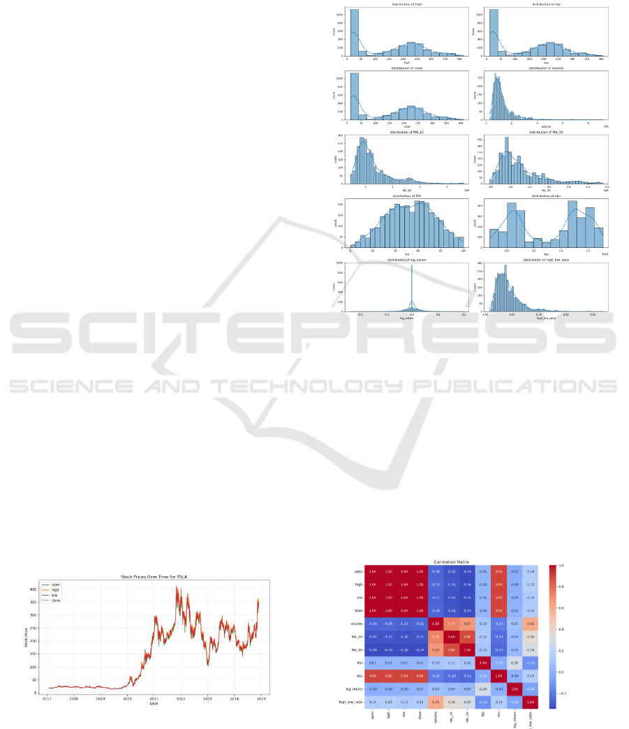
As for the Exploratory Data Analytics (EDA), a line
chart of open, high, low, close stock prices is drawn
in Figure 1. It demonstrates an increasing pattern
before 2022 and then decreases until 2024, showing a
non-stationary pattern of data.
Figure 1: Line chart for stock prices over time. (Picture
credit: Original).
In addition, the histogram graphs are
demonstrated to help understand the distribution of
data in Figure 2. It illustrates that the stock prices, RSI
and its log return are nearly normally distributed,
despite other variables do not follow the normal
distribution.
Figure 2: Histogram plot for stock prices and volume.
(Picture credit: Original).
Besides, the heatmap is also shown to illustrate
the correlation of different features used in this
dataset. It helps to visually represent the correlation
between each variable. Referred to Figure 3,
demonstrates that open, high, low, close prices are
perfectly correlated since their correlation is positive
1. MA_30 and MA_10, volume are strongly
correlated with large coefficients. Therefore, the
redundancy and multicollinearity in features should
be further considered.
Figure 3: Heatmap for features. (Picture credit: Original).
Research on Stock Price Prediction Based on Machine Learning Techniques
655
Then the Variance Inflation Factor (VIF) is used
since it quantifies the extent to which the variable's
correlation with the other variables in the model
inflates the variance of a regression line to detect
multicollinearity issue (Salmerón-Gómez et al.,
2025). A significant level of multicollinearity is
indicated if the VIF is more than 5. Since open, high,
means they are severely multicollinear, and only the
volume, RSI and high-e smallest
which less than 5.
2.2 Data Pre-processing
Then the dataset was separated into 80% for training
and 20% for testing, with the time interval shown in
Table 1.
This section must be in one column. In terms of
data preprocessing, different preprocessing
approaches are used for different models.
In terms of LR, in order to detect the
multicollinearity issue, the volume, RSI and high-low
ratio with the lowest VIF would be selected as
independent variables to satisfy the assumption of LR.
As for LSTM and GRU, since RNN is sensitive
to the scale of the input data. It is important to
standardize the data by Min-Max scaling (Jeyaraman,
2024). Then the input data is reshaped into a 3D
format suitable for these models. Using a sliding
window approach, the method extracts sequences of
mapping step lengths from the scaled data. Each
sequence, consisting of multiple time steps, is stored
in a 3D array.
By organizing the data into appropriate formats,
this integration of preprocessing enhances the
performance and accuracy of different models in
handling complex data.
Table 1: Time interval of the dataset.
Full dataset
Training dataset
Test Dataset
Time Interval
01/02/2017 29/11/2024
01/02/2017 07/05/2023
08/05/2023 29/11/2024
2.3 Linear Regression (LR)
LR is a statistical approach utilized to assess and
model the relationship between one or more predictor
variables and a response variable (Montgomery, Peck,
& Vining, 2013). LR finds the relationship of x and y
by fitting a specific linear equation with assumptions
of LR (Montgomery, Peck, & Vining, 2013). In this
project, all variables included are numerical. The
multiple linear regression describes this relationship
as shown in Equation (1).
where represents the stock prices of Tesla as the
target variable;
represents independent variable
stock closing price one day ago;
represents
independent variable two days ago;
represents
independent variable stock closing price three days
ago;
represents independent stock closing price
four days ago;
represents independent variable
stock closing price five days ago;
denotes
independent variable trading volume of the stock,
denotes independent variable RSI;
represents
independent variable ratio of high price to low price;
denotes the coefficients of variables
respectively,
denotes the intercept of the
regression plane; represents the error of residual
capturing the variance in target variable which is not
explained by LR model.
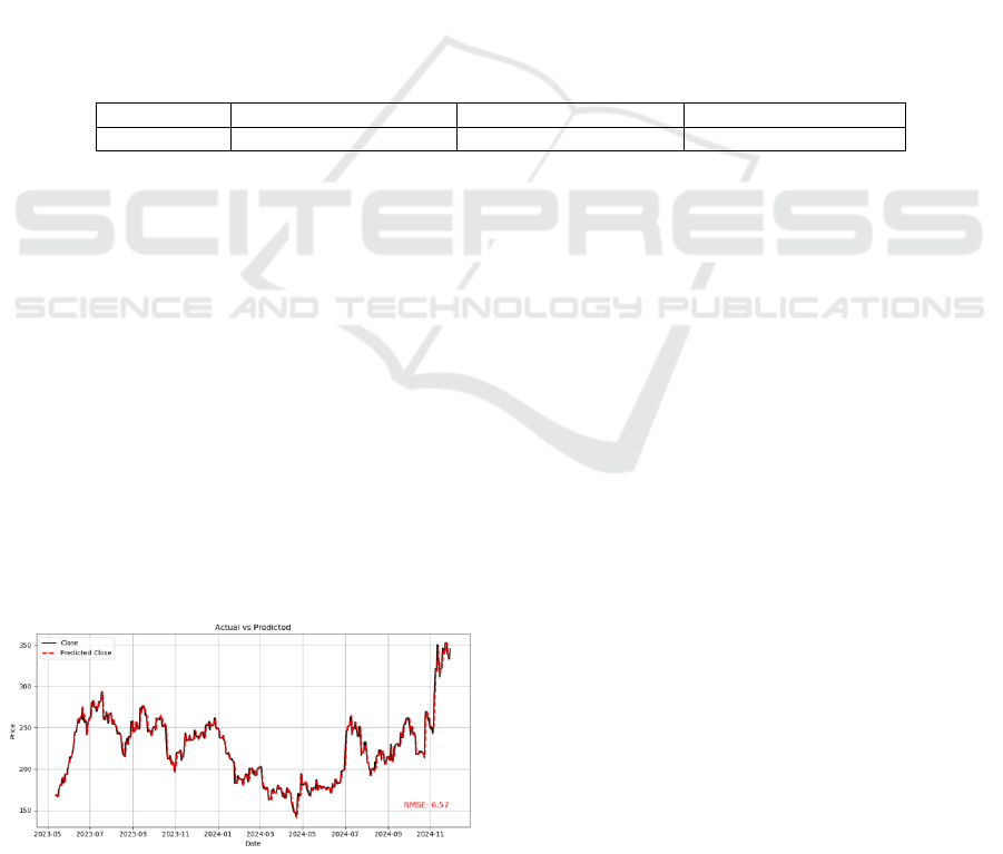
Figure 4: Actual and predicted results of Linear Regression.
(Picture credit: Original).
2.4 Long Short-Term Memory (LSTM)
LSTM network is a type of RNN capable of learning
long-term dependencies (Mim et al., 2023). The
vanishing gradient problem prevents traditional
RNNs from carrying forward information for lengthy
sequences since they only have short-term memory.
In order to solve this problem, LSTM uses memory
cells, which are managed by gates that control the
information flow and are able to retain their state
across time (Mim et al., 2023). Because they can hold
ICDSE 2025 - The International Conference on Data Science and Engineering
656
information over extended periods of time, they are
very useful for time series prediction problems.
The standard LSTM mainly consists of an input
gate shown in Equation (2), forget gate shown in
Equation (3), output gate shown in Equation (4), input
modulation gate shown in Equation (5), and memory
cell state shown in Equation (6), and the hidden state
is updated in Equation (7). One common LSTM unit
at time step t can be repressed in Equation (2) to (7).
Where the input gate, forget gate, output gate,
input modulation gate, and memory cell state are
denoted by the letters
,
,
,
, and
respectively;
and
)
denotes the sigmoid function; A hyperbolic tangent
tanh( ), while denotes an
elementwise multiplication;
is bias vector. In
particular, the forget gate
establishes the extent to
which the part of the prior
is involved in the
derivation of present
, whilst the input gate
regulates the input data's contributions for updating
the memory cell at time step t. The output gate
learns how to use the present state of the memory cell
to determine the LSTM unit's output (Shu et al.,
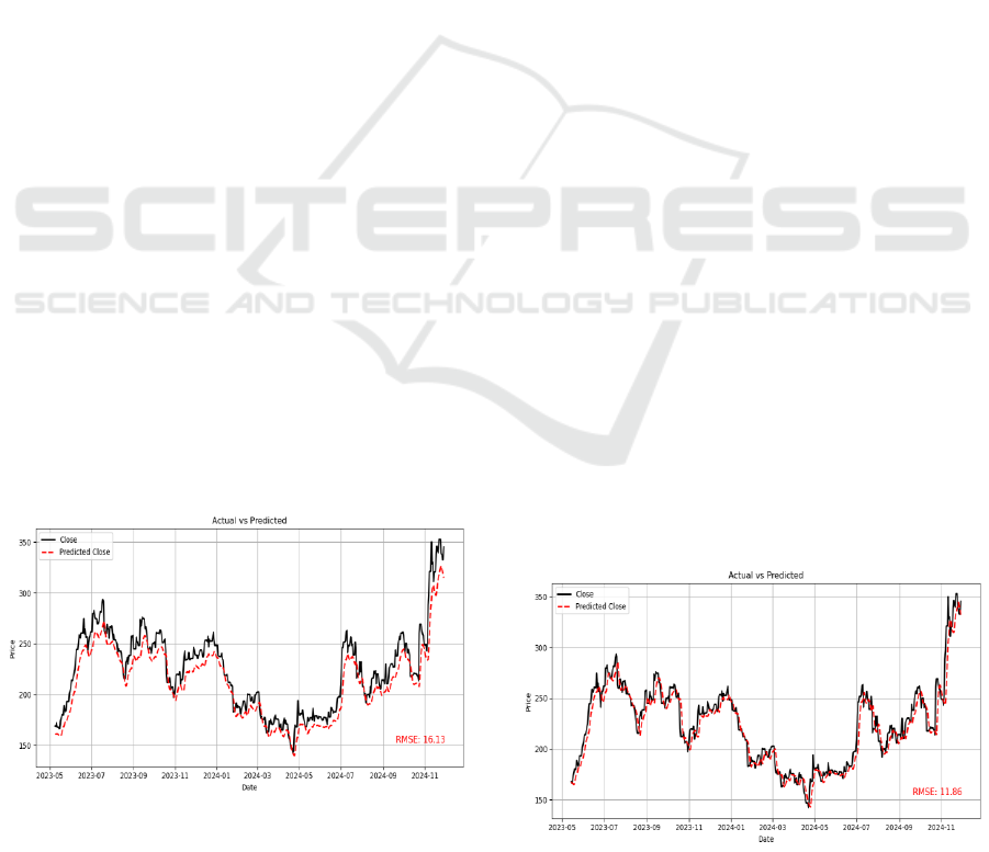
2021). And the actual stock values and predicted
values using LSTM are demonstrated in Figure 5.
Figure 5: Actual and predicted results of LSTM. (Picture
credit: Original).
2.5 Gated Recurrent Unit (GRU)
Similar to LSTM, GRU was first presented by Cho et
al. but uses a hidden state exclusively for memory
transfer and has fewer gates,
It uses two gates, the update gate z and the reset
gate r, as indicated in Equation (8), and has a similar
goal to LSTM (Pierre et al., 2023). Equation
(9) illustrates the update gate
, establishes how
much the new hidden state
is just the old state
,
and how much the new candidate state
is utilised
shown in Equation (10).
is
computed to propagate the retained information to the
subsequent unit
Figure 6: Actual and predicted results of Gated Recurrent
Unit. (Picture credit: Original).
Research on Stock Price Prediction Based on Machine Learning Techniques
657
3 RESULTS AND DISCUSSION
RMSE, MAE and R2 are used to compare the three
methodologies' effects on target variable in order to
assess these models' effectiveness. And they are all
assessed in the test data. A lower RMSE indicates a
better performance level of models and it is computed
in the following Equation (12).
Where
is the
original closing price value in
the test size,
reflects the
forecasted price and n
refers to the window size.
MAE is also called Mean Absolute Deviation. It
measures how well a model is performing by
processing the average amount that which the
forecasted values deviate from the true values (Pierre
et al., 2023). Smaller MAE values indicate that the
model's predictions are more aligned with the actual
outcomes, indicating a better performance. MAE is
expressed as the following mathematical Equation
(13).
Where n is the number of observations,
is the
actual value for the
data point in the test size,
is the predicted value for the
data point.
R2 is a key metric measuring how well the
variance in the dependent variable which can be
explained from the independent variables (Pierre et
al., 2023). A higher R2 represents a higher portion of
the variance in the dependent variable that is
predictable from the independent variables. It is
computed as well in the following Equation (14).
Where
is the original closing price in the test
size,
is referred to the predicted closing price,
is
to the mean of original closing price value.
The comparative analysis of RMSE, MAE and R2
for three different models are demonstrated in Table
2.
Table 2: Comparative analysis of RMSE, MAE and R-
Squared.
RMSE
MAE
R2
LR
6.8703
4.0410
0.9705
LSTM
15.8470
13.0769
0.8442
GRU
11.7104
8.2189
0.9142
Based on three statistical metrics, the comparative
analysis indicates that LR has the best performance
with the lowest RMSE resulting in more accurate
predictions than other models, the lowest MAE
indicating a most robust model, and the highest R2
meaning that the most time series pattern is captured
among all the models.
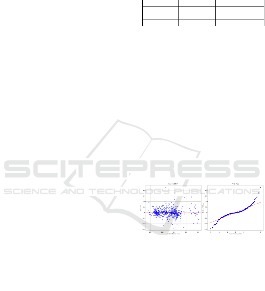
Furthermore, the residual plot and Quantile-
performance based on its assumptions shown in
Figure 7. The assumption of linearity is met because
the associations in the residual plot can be thought of
as being randomly distributed about the zero-
horizontal line, and there is no evidence to violate the
independence assumption. In terms of
homoscedasticity, the variance in the residual plot has
a constant error, so homoscedasticity is satisfied.
Because in the Quantile-Quantile Plot the points lie
along a straight line, it suggests normality of errors.
In addition, there is no multicollinearity issue since
the VIF is tested. As a result, the assumptions of LR
are all satisfied, indicating the model is likely to
produce valid, unbiased and reliable prediction results.
Figure 7: -Q plot.
(Picture credit: Original).
4 CONCLUSIONS
The objective of the article is to forecast the value of
three models: LR, LSTM, and GRU. When
comparing the techniques and their results, the best-
performing model, with the lowest RMSE and MAE,
is LR.
To briefly summarise, the dataset found from
yahoo finance is cleaned and pre-processed with
specific EDA. Then three models LR, LSTM, and
GRU are applied and compared by their performance.
ICDSE 2025 - The International Conference on Data Science and Engineering
658

Referred to several key metrics, it demonstrates that
LR has the best performance among all the models
which has the most accurate results and the most
reliable prediction.
However, it is still a challenging task to predict
stock values in a complex pattern. Beyond traditional
financial parameters, plenty of external factors impact
the financial market, such as news sentiment,
geopolitical events, and macroeconomic conditions.
Therefore, relying solely on financial features may
not fully capture the complexity of stock dynamics.
Models can perform better and offer more accurate
and robust predictions when they incorporate
additional non-financial factors, because they offer a
more thorough comprehension of the behavior of the
market. Moreover, because time series data, in which
past prices affect future prices, is not inherently taken
into account by LR, the model might not effectively
capture temporal patterns such as trends or
seasonality, which are crucial for accurate stock price
forecasting, although LR performs better than LSTM
and GRU which are able to capture temporal patterns.
In the future, incorporating additional non-
financial features such as news sentiment, macro-
economic indicators could improve the precision of
stock price forecasts. Furthermore, combining LR
and LSTM together gives an opportunity to leverage
the strengths of both techniques. It will potentially
provide a more comprehensive and accurate model
for forecasting future stock prices.
The study underscores the significant role of
machine learning in the analysis of large-scale
financial data, enhancing both the speed and
efficiency of predictions. Furthermore, machine
learning contributes to the optimization of financial
investment strategies by generating more accurate
forecasts. By mitigating human error and bias,
machine learning emerges as a critical tool in the
financial sector, facilitating informed and data-driven
decision-making processes.
REFERENCES
Cunningham, D., 2024. Tesla regains $1 trillion in market
capitalization in post-election surge. U.S. News.
Fama, E. F., MacBeth, J. D., 1973. Risk, Return, and
Equilibrium: Empirical Tests. The Journal of Political
Economy.
Ibrahim, A.W., 2024. Tesla Stock Forecasting LSTM.
Kaggle.https://www.kaggle.com/code/abdallahwagih/te
sla-stock-forecasting-lstm/notebook
Jeyaraman, B. P., 2024. Predict stock prices with LSTM
networks, 1
st
edition.
Jegadeesh, N., Titman, S., 2001. Profitability of Momentum
Strategies: An Evaluation of Alternative Explanations.
The Journal of Finance (New York).
Li, L., Wu, Y., Ou, Y., Li, Q., Zhou, Y., Chen, D., 2017.
Research on machine learning algorithms and feature
extraction for time series. 2017 IEEE 28th Annual
International Symposium on Personal, Indoor, and
Mobile Radio Communications (PIMRC).
Mim, T. R., Amatullah, M., Afreen, S., Yousuf, M. A.,
Uddin, S., Alyami, S. A., Hasan, K. F., Moni, M. A.,
2023. GRU-INC: An inception-attention based
approach using GRU for human activity recognition.
Expert Systems with Applications.
Montgomery, D. C., Peck, E. A., Vining, G. G., 2013.
Introduction to linear regression analysis, Wiley. 5
th
edition.
Tesla Stock Price Prediction using GRU
Tutorial.Kaggle.
Pierre, A. A., Akim, S. A., Semenyo, A. K., Babiga, B.,
2023. Peak Electrical Energy Consumption Prediction
by ARIMA, LSTM, GRU, ARIMA-LSTM and
ARIMA-GRU Approaches. Energies (Basel).
Shu, X., Zhang, L., Sun, Y., Tang, J., 2021. Host-Parasite:
Graph LSTM-in-LSTM for Group Activity Recognition.
IEEE Transaction on Neural Networks and Learning
Systems.
Vijh, M., Chandola, D., Tikkiwal, V. A., Kumar, A., 2020.
Stock Closing Price Prediction using Machine Learning
Techniques. Procedia Computer Science.
Salmerón-Gómez, R., García-García, C. B., García-Pérez,
J., 2025. A Redefined Variance Inflation Factor:
Overcoming the Limitations of the Variance Inflation
Factor: A Redefined Variance Inflation Factor.
ComputationalEconomics.
Research on Stock Price Prediction Based on Machine Learning Techniques
659
