Stock Price Prediction Based on Linear Regression and Significance

Analysis

Shengzhou Li

Faculty of Mathematics, University of Waterloo, Waterloo, Ontario, Canada

Keywords: Stock Prediction, Linear Regression, Lagged Features, F-Test. Feature Importance.

Abstract: Accurate stock price prediction is fundamental to financial market efficiency, enabling informed trading

strategies and systemic risk mitigation in increasingly volatile global markets. To address the critical yet

underexplored issue of feature selection efficacy, this paper investigates stock price prediction for Apple Inc.

(AAPL) over the 2013–2018 period by applying a linear regression model and analyzing four fundamental

price features (open, high, low, close) along with their five-day lags. Single-group and combined-group

approaches were applied to forecast next-day and five-day-ahead closing prices. The aim was to clarify which

feature combination offers greater predictive benefit. Results show that while a single-group model relying

on closing prices alone performs relatively well, its accuracy does not significantly differ from the combined

model. This finding suggests that feature redundancy may reduce potential gains in short-term contexts.

Meanwhile, the partial F-test indicates that high price features exhibit notable statistical significance for

capturing market peaks and volatility, whereas information from open, low, and close can be partially

overlapped by other variables.

1 INTRODUCTION

The stock market is a trading venue where investors

buy and sell shares based on availability, and its

fluctuations directly influence profits: a rise in prices

generates returns, whereas a downturn leads to losses

(Ghania, Awaisa, & Muzammula, 2019). Machine

learning, as a branch of artificial intelligence, enables

computers to learn from data without explicit

instructions, relying instead on patterns extracted

from past observations (Emioma & Edeki, 2021).

Predicting stock prices has long been considered both

adventurous and engaging, particularly because it

involves monetary risk. This demand for forecasting

has spurred diverse approaches, each striving to

identify influential factors and refine predictive

capabilities. Among these methods, a key principle

for accuracy is learning from historical examples,

allowing a system to derive rules and make decisions

more effectively. Consequently, machine learning

techniques, whether supervised or unsupervised,

provide a powerful means of capturing and applying

knowledge from past instances to enhance stock

market predictions (Pahwa et al., 2017).

https://orcid.org/0009-0005-1812-409X

Stock market prediction has been recognized as

both challenging and important because of price

volatility and nonlinear patterns. Earlier research

showed the significant impact of market shifts,

especially during the 2008 crash when the Dow Jones

Industrial Average dropped sharply, highlighting the

need for robust forecasting methods (Panwa et al.,

2021). Traditional and newer machine learning

approaches, such as artificial neural networks (ANN)

and random forests (RF), have been explored in depth

to improve accuracy. ANN captures detailed price

patterns through multi-layer designs, while RF helps

reduce overfitting and refine feature importance via

ensemble learning (Rouf et al., 2021; Nikou et al.,

2019; Vijh et al., 2020). Deep learning methods like

long short-term memory (LSTM) networks build on

these advantages by addressing temporal factors,

allowing them to surpass ANN and SVM in time-

series forecasting (Nikou et al., 2029). Recent work

also stresses feature engineering: when extra

variables derived from standard price data (Open,

High, Low, Close) are added, machine learning

models achieve lower RMSE and MAPE in volatile

markets (Rouf et al., 2021; Vijh et al., 2020) .

596

Li, S.

Stock Price Prediction Based on Linear Regression and Signiﬁcance Analysis.

DOI: 10.5220/0013702600004670

Paper published under CC license (CC BY-NC-ND 4.0)

In Proceedings of the 2nd International Conference on Data Science and Engineering (ICDSE 2025), pages 596-603

ISBN: 978-989-758-765-8

Meanwhile, notes that linear regression can

outperform SVM in specific supervised learning

contexts, indicating that model and feature choices

should align with the characteristics of each market

(Panwar et al., 2021).

This study focuses on the core challenge of

feature selection and model interpretability in stock

price prediction, aiming to address the following key

scientific questions. First, in a linear regression model

incorporating either a single feature group or a

combination of multiple feature groups, which

configuration demonstrates greater predictive

advantage for medium-term (five-day-ahead) stock

prices? Second, if all features are included in a unified

model, can the stepwise removal of individual price

feature groups using the grouped F-test effectively

reveal their overall contribution and statistical

significance within the model? By comparing the

predictive performance of single-group and multi-

group feature models and assessing feature group

importance in a comprehensive model, this study

seeks to provide targeted empirical evidence to

enhance the application of linear regression in stock

market prediction.

2 DATA AND EXPLORATORY

DATA ANALYSIS

We strongly encourage authors to use this document

for the preparation of the camera-ready. Please follow

the instructions closely in order to make the volume

look as uniform as possible (Moore and Lopes, 1999).

Please remember that all the papers must be in

English and without orthographic errors.

Do not add any text to the headers (do not set

running heads) and footers, not even page numbers,

because text will be added electronically.

For a best viewing experience the used font must

be Times New Roman, on a Macintosh use the font

named times, except on special occasions, such as

program code (Section 2.3.8).

2.1 Data Source and Description

The dataset used in this study comes from the publicly

available "S&P 500" dataset on Kaggle. This dataset

contains historical market data for the constituent

stocks of the S&P 500 index, covering the period

from February 8, 2013, to February 7, 2018. Due to

the high volatility and research value of the

technology sector, this study selects Apple Inc.

(AAPL) as the specific empirical research object.

After importing and filtering the data, this study

obtains the daily market data table of AAPL within

the above-mentioned time range, as shown in Table 1

(only partial fields are displayed). The dataset

includes data (trading date), open (opening price of

the day), high (highest price of the day), low (lowest

price of the day), close (closing price of the day),

volume (trading volume of the day), and Name (stock

name). A total of 1,259 records are included, covering

Apple Inc.'s stock market data from February 8, 2013,

to February 7, 2018.

Table 1: AAPL stock data sample.

date open high low close volume Name

1259 2013-02-08 67.7142 68.4014 66.8928 67.8542 158168416 AAPL

1260 2013-02-11 68.0714 69.2771 67.6071 68.5614 129029425 AAPL

1261 2013-02-12 68.5014 68.9114 66.8205 66.8428 151829363 AAPL

1262 2013-02-13 66.7442 67.6628 66.1742 66.7156 118721995 AAPL

1263 2013-02-14 66.3599 67.3771 66.2885 66.6556 88809154 AAPL

2.2 Data Pre-processing

This study first evaluates data quality using the

pandas library in Python, employing the isnull().

sum() method to detect missing values in key features

such as opening price, closing price, highest price,

lowest price, and trading volume. The statistical

results indicate that all features have zero missing

values, achieving a data completeness rate of 100%.

Therefore, no missing value imputation is performed.

Subsequently, to establish a supervised learning

framework, the short-term price prediction target is

defined as the closing price five days ahead

(Close_5days_ahead). The pandas.DataFrame.shift(-

5) function is applied to shift the closing price series

forward by five trading days, aligning the current

row's features with the closing price five days later.

Stock Price Prediction Based on Linear Regression and Signiﬁcance Analysis

597

Next, lagged features for (open, close, high, low)

are constructed for the past 1 to 5 days. Specifically,

for each price indicator 𝑋



( 𝑋∈



𝑂𝑝𝑒𝑛,𝐶𝑙𝑜𝑠𝑒,𝐻𝑖𝑔ℎ,𝐿𝑜𝑤



), the shift(t) operation

generates lagged features X





=𝑋



,𝑡∈



1,2,3,4,5



. Each lagged feature X_lag_k represents

"the value of X k days ago". These lagged columns

allow the regression model to quantify the influence

of historical price information over a period on the

current or future closing price.

Finally, in the feature engineering process, the

lagging operation results in five missing rows at the

beginning of the sequence. These initial missing

values are removed using the

pandas.DataFrame.dropna() function, ultimately

yielding 1254 valid samples. The preprocessed

dataset provides a reliable foundation for subsequent

regression model training and feature importance

analysis, with a structure that meets the requirements

of supervised learning tasks.

2.3 Exploratory Data Analysis

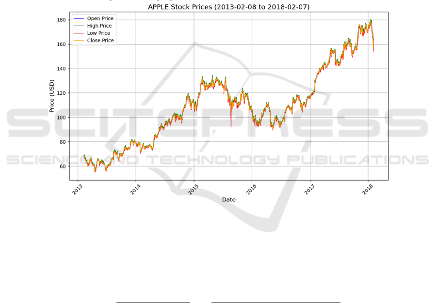
To better visualize Apple's stock price performance

and volatility over the study period, Figure 1 plots the

trends of the opening price, highest price, lowest

price, and closing price over time. From 2013 to

2018, AAPL exhibits an overall upward trend, with

multiple instances of significant short-term

fluctuations or pullbacks, reflecting the combined

influence of market sentiment and macroeconomic

conditions.

Figure 1: The trends of different AAPL price fields over time. (Picture credit: Original)

Based on this, to examine the potential

relationship between stock price fluctuations and

trading volume, as well as the intrinsic weighting of

daily return variations, this study constructs a

volume-weighted daily return indicator 𝑅



, as defined

in Equation (1).

𝑅



=

𝐶𝑙𝑜𝑠𝑒



−𝐶𝑙𝑜𝑠𝑒



𝐶𝑙𝑜𝑠𝑒





𝑉𝑜𝑙𝑢𝑚𝑛



−min



𝑉𝑜𝑙𝑢𝑚𝑛



max



𝑉𝑜𝑙𝑢𝑚𝑛



−min



𝑉𝑜𝑙𝑢𝑚𝑛









This indicator further illustrates the time series of

the "weighted daily growth rate". It first measures the

relative daily price fluctuation and then applies

weighting based on the trading volume of the day,

thereby emphasizing the impact of trading days with

both high volume and significant price changes on

overall volatility. It can be observed that if a trading

day experiences a notable increase or decrease in

price accompanied by high trading volume, the

weighted growth rate of that day becomes more

pronounced. This indicates that such trading days

carry greater weight or influence on stock price

movements. Figure 2 shows the trend of AAPL's

weighted daily growth rate over time.

ICDSE 2025 - The International Conference on Data Science and Engineering

598

Figure 2: AAPL weighted daily growth rate over time. (Picture credit: Original)

Analyzing the information reflected in Figures 1

and Figure 2 allows for a preliminary grasp of the

long-term evolution trajectory of Apple's stock price

and identifies key volatility periods. Additionally, the

weighted growth rate helps recognize trading days

where price fluctuations are more closely associated

with changes in trading volume. Building on this

foundation, the subsequent research will focus on

historical prices and their lagged features to construct

a more comprehensive predictive model and

quantitatively explore the influence of various

features on future stock prices.

3 METHODOLOGY

3.1

Overall Proces

Figure 3: Overall Process. (Picture credit: Original)

This study follows a standardized experimental

process based on Apple's (AAPL) historical stock

price data. It extracts the opening price, closing price,

highest price, and lowest price to construct the basic

feature set, handles missing values using adjacent

mean imputation, and generates 1–5 day lagged

features. Invalid samples are then removed, and the

dataset is split into a training set (80%) and a test set

(20%) in chronological order. A linear regression

framework is employed to train both a full-feature

model and four constrained models separately.

Prediction performance differences are evaluated

using R² and MSE, while the partial F-test is used to

quantify the significance of feature groups.

Ultimately, a multidimensional feature importance

evaluation system is established. Figure 3 shows the

overall process.

3.2 Linear Regression Model

Regression analysis is performed so as to determine

the correlations between two or more variables

having cause and effect relations, and to make

predictions for the topic by using the relation (Uyanık

& Güler, 2013). In the basic linear regression model,

the relationship between the target variable y and

multiple features x_1, x_2, ⋯, x_n is expressed as

shown in Equation (2).

𝑦= 𝛽



+𝛽



𝑥



+𝛽



𝑥



+⋯+𝛽



𝑥



+𝜖





Here, 𝛽



represents the intercept, 𝛽



are the

regression coefficients for each feature, and 𝜀 denotes

the random error term. This model assumes that the

impact of features on the target variable is linear, and

it requires the error terms to be independently and

identically distributed with constant variance. In

practical applications, linear regression is widely used

Stock Price Prediction Based on Linear Regression and Signiﬁcance Analysis

599

due to its simplicity and strong interpretability.

However, when there is significant nonlinearity

between features and the target variable, or when

strong multicollinearity exists among features, the

model's predictive performance and coefficient

stability may be affected (Montgomery, Peck, &

Vining, 2021).

3.3 Experimental Design and Feature

Combinations

In this study, the experiment for predicting future

closing prices is designed by comparing regression

models with different feature combinations from

three perspectives.

Separate models are built to use the opening price,

closing price, highest price, and lowest price of the

current day and the past five days to predict the

closing price of the next day or five days later. Each

model uses only the same type of price data and

predicts the closing price five days later using a linear

regression method.

The combined feature model builds upon this by

incorporating open, close, high, low along with their

respective 1–5 day lagged features into a larger

model. This allows for an evaluation of the

improvement in predictive ability when all price

information is included together, as well as the

potential impact of multicollinearity.

To further quantify the contribution of each

feature group within the overall model, this study

employs a grouped feature removal approach.

Starting with a model that includes all features, each

feature group is sequentially removed. Then observe

the change in model performance after removing a

group, if performance declines significantly, it

indicates that the removed feature group plays an

important role in prediction; conversely, if the

performance remains stable, the feature group’s

impact is likely limited.

Through this multi-level experimental design, the

study systematically examines the role of different

price feature groups in predicting the closing price on

the next day or five days ahead. This structured

approach provides a clear framework for the

subsequent grouped F-test and model interpretation.

3.4 Partial F-Test

The Partial F-Test is a statistical method used to

evaluate whether a specific group of feature variables

contributes significantly to the predictive ability of a

regression model. The core idea is to compare the

goodness-of-fit between an unrestricted model and a

restricted model to determine whether the removal of

that feature group significantly degrades model

performance (Duncan, 1955).

3.5 Testing Steps and Implementation

3.5.1 Model Construction

The unrestricted model includes all feature groups

(opening price, closing price, highest price, lowest

price, and their lagged terms) along with a constant

term and is fitted using Ordinary Least Squares

(OLS). The model is formulated as shown in Equation

(3).

𝑦



=𝛽



+𝛽



𝑥







+𝜖





Here, 𝑦



represents the prediction target

(closing price five days ahead), 𝑥



denotes the feature

variables, and 𝛽



are the corresponding coefficients.

The restricted model sequentially removes a

specific feature group (e.g., the open price group,

including open and its lagged terms), retaining only

the remaining three groups and refitting the model. In

this case, the degrees of freedom decrease, but the

explanatory power of the remaining features is

preserved.

3.5.2 Statistical Calculation

By comparing the Residual Sum of Squares (RSS) of

the unrestricted model and the restricted model, the

F-statistic can be computed. The specific process is

formulated as shown in Equation (4).

𝐹=

𝑅𝑆𝑆



−𝑅𝑆𝑆



𝑞

⁄

𝑅𝑆𝑆





𝑛−𝑘−1

⁄





Here, 𝑅𝑆𝑆



and 𝑅𝑆𝑆



represent the RSS for

the unrestricted model and restricted model,

respectively; 𝑞 denotes the number of removed

features (each group in this study contains six

features, the current day's price + five lagged terms);

𝑛 is the sample size; 𝑘 is the total number of features

in the unrestricted model (24 features + a constant

term); the degrees of freedom for the F-test is



𝑞,𝑛 − 𝑘 − 1



3.6 Evaluation Metrics

This study employs two types of metrics to evaluate

model performance. R² measures the proportion of

variance in the target variable explained by the model,

ICDSE 2025 - The International Conference on Data Science and Engineering

600

with values closer to 1 indicating better fit. Mean

Squared Error (MSE) calculates the average squared

error between predicted and actual values, reflecting

the absolute error level of the model.

The dataset is split chronologically into a training

set (first 80%) and a test set (last 20%). This

partitioning prevents future data leakage and aligns

with the nature of financial time-series forecasting,

ensuring that the model relies only on historical data

to predict future values, thereby enhancing the

realism of the evaluation.

4. Experimental Results and Analysis

4.1 Experimental Data Analysis

Tables 2 and 3 present the regression model

performance based on individual price features. The

model using close prices and their lagged features

achieved a relatively high 𝑅



(0.8847) and a lower

MSE (17.0267) when predicting the closing price five

days ahead. This indicates that among individual

price categories, recent closing price information has

stronger explanatory power for future stock

movements. In contrast, the open price group

performed relatively worse (𝑅



=0.8666), suggesting

that the opening price may be less reliable for short-

term prediction compared to the closing price. None

of the single-variable models achieved an 𝑅



exceeding 0.89, indicating an inherent limitation in

predictive power when relying solely on a single price

dimension.

Table 2: Single-Variable Linear Regression Coefficients.

Coefficient High Low Close Open

Intercept 1.3860 1.6276 1.5169 1.6291

𝑿

𝒕

1.1270 0.9251 0.9533 0.8338

𝑿

𝒕𝟏

-0.1568 -0.0388 -0.0232 0.1799

𝑿

𝒕𝟐

0.1125 0.0524 0.0597 -0.0219

𝑿

𝒕𝟑

-0.0322 -0.0213 -0.0109 0

𝑿

𝒕𝟒

0.0357 0.1262 0.0519 0.0656

𝑿

𝒕𝟓

-0.1058 -0.0477 -0.0429 -0.0765

Table 3: Single-Variable Linear Regression Performance

Comparison.

feature

R² MSE

High 0.8763 18.2807

Low 0.8809 17.5988

Close 0.8847 17.0267

en 0.8666 19.7848

Table 2 present single-variable linear regression

coefficients. Table 3 presents

single-variable linear

regression performance comparison.

Table 4 presents the

overall accuracy of the model after incorporating all

features ( 𝑅



=0.8844 ， MSE=17.0805). The

performance is not significantly different from the

best-performing individual feature group model

(Close group), which may be attributed to

multicollinearity or redundant information among

highly correlated features. This suggests that a single

price type holds considerable weight in medium-term

forecasting, and feature aggregation does not yield

the expected performance gain.

Table 4: Prediction Results with All Features Combined.

𝑅



0.8844

MSE 17.0805

As shown in Table 5, the changes in 𝑅



and MSE

after removing different feature groups are relatively

small. For example, when the open group is removed,

𝑅



=0.8839 and MSE = 17.1528, showing little

difference compared to other excluded groups. This

indicates that eliminating a single feature group does

not significantly degrade overall predictive

performance, reflecting the complementary nature of

different price features. Notably, after removing the

close group, the model's performance remains almost

unchanged, which contradicts its optimal

performance in single-variable regression. This

suggests that the information contained in close may

be partially captured by other features.

Table 5: Impact of Removing Feature Groups on Model

Performance.

Model name

𝑅



MSE

Without o

rou

0.8839 17.1528

Without close

rou

0.8844 17.0849

Without high group 0.8838 17.1720

Without low group 0.8831 17.2677

As shown in Table 6, the grouped F-test results

indicate that only the high group exhibits statistical

significance at the α=0.05 level. This suggests that

when all features are used together, the highest price

Stock Price Prediction Based on Linear Regression and Signiﬁcance Analysis

601

and its lagged information play a more critical role in

model fitting. The p-values for the remaining groups

are all greater than 0.05, implying that from a

statistical testing perspective, removing these groups

does not significantly deteriorate the model's

performance. This highlights that strong individual

feature group performance does not necessarily imply

high marginal contribution when combined with

other features. Conversely, although the high group

did not stand out in single-feature predictions, it

provides an irreplaceable incremental effect in the full

model.

Table 6: Feature Group Significance Test Results.

Feature F-value p-value

Significance test results（α=0.05）

en 0.309 0.932 No Si

nificant Contribution

(

Null H

othesis Retained

)

Close 1.703 0.117 No Si

nificant Contribution

(

Null H

othesis Retained

)

High 3.420 0.002 Significant Contribution (Null Hypothesis Rejected)

Low 0.979 0.438 No Significant Contribution (Null Hypothesis Retained)

The observed differences suggest that while

different price features may have similar impacts on

model accuracy in medium-term predictions, their

complementarity and interactions in larger models

require deeper examination through grouped removal

or grouped F-tests. For features like closing price,

which demonstrate strong standalone predictive

power, their contribution may not remain the most

significant when combined with all other information.

In contrast, high price may exhibit unique advantages

in capturing market peaks and volatility ranges,

leading to more pronounced statistical gains. Overall,

these findings highlight that in practical applications,

feature selection and evaluation should be tailored to

specific model objectives and market dynamics,

ensuring that different price groups are assessed

flexibly for their predictive importance.

5 CONCLUSIONS

This study centres on the linear regression model,

examining the performance of individual feature

groups versus multiple feature combinations in

medium-term (five-day-ahead) predictions and

evaluating the contribution of each feature group

using the grouped F-test. The results indicate that

while the closing price group performed relatively

well in single-variable models, its accuracy did not

significantly surpass that of the combined model,

suggesting that variable redundancy may reduce the

benefits of incorporating multiple features.

Meanwhile, the high price group exhibited statistical

significance in the grouped F-test, indicating its

irreplaceable value in capturing market peaks and

volatility ranges, whereas the information contained

in the closing price, opening price, and lowest price

groups may have been partially covered by other

features. These findings address the two core research

questions: first, the difference between single-group

and multi-group features in short- to medium-term

predictions is limited, with the closing price group

performing comparably to the combined model;

second, the highest price group demonstrating a

distinct contribution to the overall model, as

confirmed by the grouped F-test. It is important to

note that this study is based solely on AAPL stock and

employs linear regression, which may not fully

account for time-series autocorrelation and nonlinear

limitations. Future research could integrate additional

features (e.g., trading volume, financial indicators,

news sentiment) and extend the analysis to multiple

stocks, while also exploring nonlinear models such as

random forests or LSTM to enhance adaptability to

market fluctuations and deepen the study of stock

market prediction.

REFERENCES

Duncan, D. B. (1955). Multiple range and multiple F tests.

Biometrics, 11(1), 1-42.

Emioma, C. C., & Edeki, S. O. (2021). Stock price

prediction using machine learning on least-squares

linear regression basis. In Journal of Physics:

Conference Series (Vol. 1734, No. 1, p. 012058). IOP

Publishing.

Ghania, M. U., Awaisa, M., & Muzammula, M. (2019).

Stock market prediction using machine learning (ML)

algorithms. ADCAIJ: Advances in Distributed

Computing and Artificial Intelligence, 8(4), 97-116.

Montgomery, D. C., Peck, E. A., & Vining, G. G. (2021).

Introduction to linear regression analysis. John Wiley

& Sons.

Nikou, M., Mansourfar, G., & Bagherzadeh, J. (2019).

Stock price prediction using DEEP learning algorithm

and its comparison with machine learning algorithms.

Intelligent Systems in Accounting, Finance and

Management, 26(4), 164-174.

Pahwa, N., Khalfay, N., Soni, V., & Vora, D. (2017). Stock

prediction using machine learning a review paper.

ICDSE 2025 - The International Conference on Data Science and Engineering

602

International Journal of Computer Applications,

163(5), 36-43.

Panwar, B., Dhuriya, G., Johri, P., Yadav, S. S., & Gaur, N.

(2021, March). Stock market prediction using linear

regression and SVM. In 2021 International Conference

on Advance Computing and Innovative Technologies

in Engineering (ICACITE) (pp. 629-631). IEEE.

Rouf, N., Malik, M. B., Arif, T., Sharma, S., Singh, S.,

Aich, S., & Kim, H. C. (2021). Stock market prediction

using machine learning techniques: a decade survey on

methodologies, recent developments, and future

directions. Electronics, 10(21), 2717.

Uyanık, G. K., & Güler, N. (2013). A study on multiple

linear regression analysis. Procedia-Social and

Behavioral Sciences, 106, 234-240.

Vijh, M., Chandola, D., Tikkiwal, V. A., & Kumar, A.

(2020). Stock closing price prediction using machine

learning techniques. Procedia Computer Science, 167,

599-606.

Stock Price Prediction Based on Linear Regression and Signiﬁcance Analysis

603