Observation-Based Inverse Kinematics for Visual Servo Control

Daniel Nikovski

Mitsubishi Electric Research Labs, Massachusetts, U.S.A.

Keywords:

Robotics, Learning Control, Conﬁguration Learning, Visuomotor Policies.

Abstract:

We propose a method for estimating the joint conﬁguration of articulated mechanisms without joint encoders

and with unknown forward kinematics, based solely on RGB-D images of the mechanism captured by a

stationary camera. The method collects a sequence of such images under a suitable excitation control policy,

extracts the 3D locations of keypoints in these images, and determines which of these points must belong

to the same link of the mechanism by means of testing their pairwise distances and clustering them using

agglomerative clustering. By computing the rigid-body transforms of all bodies with respect to the keypoints’

positions in a reference image and analyzing each body’s transform expressed relative to all other bodies’

coordinate reference frames, the algorithm discovers which pairs of bodies must be connected by a single-

degree-of-freedom joint and based on this, discovers the ordering of the bodies in the kinematic chain of the

mechanism. The method can be used for pose-based visual servocontrol and other robotics tasks where inverse

kinematics is needed, without providing forward kinematics or measurements of the end tool of the robot.

1 INTRODUCTION

Humans and animals possess remarkable abilities to

execute very complex motions based on sensory ob-

servations, starting from hunting for prey and avoid-

ing predators and ranging to precise motion such as

hitting a fast moving ball with a bat or assembling

a complex electronic device. Over the course of mil-

lions of years of evolution, one sensory modality – vi-

sion – has provided an overwhelming advantage when

performing such motions, and modern control engi-

neering and artiﬁcial intelligence (AI) have sought to

emulate computationally the abilities of living organ-

isms to interpret visual data for the purpose of direct-

ing intelligent behavior. This effort, combined with

the ever decreasing cost and increasing performance

of high-resolution cameras and compact embedded

micro-controllers, has brought about a generational

change in robotics, where rigidly-programmed robots

executing identically repeated motions are gradually

being replaced by robots that can interpret visual in-

put and adjust their motion accordingly.

However, this transition is associated with the cost

of manually developing an observer of the system

under control, employing computer vision and con-

trol engineering techniques (Szeliski, 2022; Franklin

et al., 2015). It is thus very appealing economically

https://orcid.org/0000-0003-2919-645X

to automate the process of constructing observers for

nonlinear systems based on visual observations. The

ﬁeld of state representation learning (SRL) for control

addresses the general problem of producing compact

descriptors of the state of a dynamical system from

observation data and their use for designing control

policies (Lesort et al., 2018). Methods proposed in

the closely related ﬁeld of nonlinear system identi-

ﬁcation also often construct state representations as

their byproducts (Nelles, 2020). However, general

methods in these ﬁelds, almost exclusively based on

machine learning algorithms, often suffer from very

high sample complexity, i.e., they need to see very

many training examples in order to learn a suitable

model and/or state representation, often limiting their

applicability to relatively simple systems with few in-

dependent state variables. Moreover, such methods

tend to produce state representations where the contri-

butions of the individual state variables are conﬂated.

This is in contrast with the traditionally hand-crafted

perception modules in AI, where a scene descriptor

is usually factored into the states of the objects the

scene consists of, or state vectors in control systems

engineering, which are similarly a concatenation of

the states of the system’s individual components.

It is thus highly desirable to be able to construct

from training data useful state representations that are

factored across a set of moving objects that exist in a

200

Nikovski, D.

Observation-Based Inverse Kinematics for Visual Servo Control.

DOI: 10.5220/0013701100003982

Paper published under CC license (CC BY-NC-ND 4.0)

In Proceedings of the 22nd International Conference on Informatics in Control, Automation and Robotics (ICINCO 2025) - Volume 1, pages 200-207

ISBN: 978-989-758-770-2; ISSN: 2184-2809

scene corresponding to a controllable system in mo-

tion. An example of such a system is an articulated

robot arm consisting of several rigid bodies (links)

connected to one another by means of joints. The

links are arranged in a kinematic chain and the joints

connecting them can be translational or rotational.

Most industrial manipulators ﬁt this deﬁnition.

Other examples are cranes (gantry, boom, beam,

etc.) whose mechanism varies depending on what

kind of joints are used. Automatic control of in-

dustrial manipulators has been researched over many

decades (Siciliano and Khatib, 2016), and automation

of cranes has also advanced in recent years (Mojal-

lizadeh et al., 2023). Owing to their second-order

dynamics, the state of such mechanisms can be ex-

pressed as the set of joint positions (angles or dis-

placements) as well as their velocities.

Although the joint positions of many articulated

mechanisms can be measured by means of encoders,

in other cases, for example for the cables hoisting the

load of a crane, this is not feasible. An alternative is

to implement an estimator based on visual data and

it is desirable to automate this process. We propose

one such algorithm for conﬁguration descriptor con-

struction from image data. The main insight behind

it is that if we can reliably detect and track 3D key-

points in sequences of such images, we can recover

the mechanism’s conﬁguration much more easily than

if we were working with the raw pixels in the im-

ages. Section 2 describes the problem setting and the

assumptions about visual data we make, and section

3 describes some approaches to solving the problem.

Section 4 describes our proposed method and Section

5 presents its empirical veriﬁcation. Section 6 pro-

poses future directions and concludes.

2 PROBLEM DEFINITION

We are interested in the accurate estimation of the

conﬁguration of an articulated mechanism, such as

a robot arm, entirely from camera images, and the

use of this conﬁguration estimate for the purposes of

control of the mechanism. The mechanism comprises

an unknown number of rigid bodies connected in a

kinematic chain via single-degree-of-freedom (DoF)

joints, whose types – either prismatic or revolute –

are not known a priori. Furthermore, the size, appear-

ance, and ordering of the rigid bodies within the chain

are also unknown, precluding direct recovery of the

mechanism’s true state. However, if a conﬁguration

representation can be derived from visual data that is

equivalent to the true conﬁguration – i.e., it maintains

a one-to-one correspondence – then state-based con-

trol techniques can still be employed for effective con-

trol of the mechanism.

We consider a set S of N distinctive 3D keypoints

tracked over T time steps, yielding measurements of

the form p

= [x

]

for i = 1, ..., N and k =

1,. .. ,T . The collection of keypoint measurements at

time k is denoted by the matrix P

= [p

]

∈ R

N×3

These 3D positions can be estimated using an RGB-

D camera that captures a sequence of T frames while

the mechanism is actuated under a persistently excit-

ing control policy. Distinctive features, such as cor-

ners, are extracted from the RGB images (Szeliski,

2022), and their 3D positions are computed in the

camera frame using the corresponding depth data and

the camera’s intrinsic parameters. We do not assume

continuous visibility of all keypoints; some may be

occluded at certain time steps, resulting in missing

data. Moreover, the visible keypoints are subject to

measurement noise due to pixel quantization, lim-

ited depth resolution, and potential mechanical dis-

turbances. Finally, we assume that the number of

keypoints N signiﬁcantly exceeds the number of rigid

bodies n, ensuring that each body is associated with

at least four, and preferably more, visible keypoints to

enable reliable pose estimation in the camera frame.

Given the (potentially sparse) data tensor P =

] ∈ R

N×T ×3

, where k = 1,...,T , our objective is to

infer the underlying structure and motion of the artic-

ulated mechanism. Speciﬁcally, we aim to determine:

(i) the number of rigid bodies present in the scene;

(ii) the assignment of each of the N keypoints to their

corresponding rigid body; (iii) the pose of each body

relative to a reference pose at every time step; (iv)

the connectivity structure of the mechanism, identi-

fying which bodies are linked via single-DoF joints;

and (v) the joint conﬁgurations over time, expressed

relative to a reference joint position. The reference

body poses are deﬁned with respect to a chosen time

step, such as the initial frame in the sequence, when

the reference joint positions are assumed to be zero.

At run time, we aim to bring the mechanism to

a goal state speciﬁed implicitly by means of an im-

age of the mechanism in the desired goal state, as

is customary in the ﬁeld of visual servocontrol (VS)

(Chaumette et al., 2016). Using steps (iii) and (v)

above and the mechanism structure discovered in

steps (i), (ii), and (iv), we estimate the desired goal

joint state. Then, we control the articulated mecha-

nism by repeatedly (a) capturing an RGB-D image of

the mechanism; (b) determining the 3D positions of

the keypoints in it; (c) computing the pose of each

body with respect to the reference pose, analogously

to step (iii) in the analysis stage above; (d) comput-

ing the joint conﬁguration at this time, again analo-

Observation-Based Inverse Kinematics for Visual Servo Control

201

gously to step (v) above; (e) computing a feedback

error with respect to the desired goal conﬁguration, in

estimated joint space; and (f) computing a control sig-

nal based on the feedback error that aims to bring the

error to zero, using a suitable control method, such as

proportional-integral-derivative (PID) control.

3 RELATED WORK

Some deep reinforcement learning (DRL) algorithms

have achieved several successes in learning visuo-

motor control policies directly in terms of high-

dimensional observations, including camera images,

but these typically require millions of exprimental tri-

als. There do exist some DRL algorithms with ac-

ceptable sample complexity that can be trained on real

robotic hardware, but not quite matching the problem

we are interested in. For example, the Guided Policy

Search (GPS) algorithm has been able to learn control

policies for various difﬁcult robotics tasks (Levine

et al., 2016). However, this algorithm did have ac-

cess to the true low-dimensional state of the system

to compute optimal state-based policies at training

time, later turning these policies into observation-

based ones using supervised learning. In contrast, we

do not assume access to the true state at any time.

Image-based visual servocontrol (IBVS) algo-

rithms could be very effective, but usually assume that

all features will be visible at all times, otherwise they

would fail (Chaumette et al., 2016). Another class of

VS algorithms known as pose-based visual servocon-

trol (PBVS) algorithms operate by ﬁrst estimating the

current state of the mechanism from images, essen-

tially equivalent to estimating its conﬁguration, fol-

lowed by conventional control in joint space. How-

ever, this cannot be done analytically without a kine-

matic model of the mechanism and knowledge of how

it would look like in different conﬁgurations. An al-

ternative is to apply SRL to learn compact represen-

tations of the controlled system, including articulated

mechanisms, and use these representations for vari-

ous control and decision-making tasks, such as VS for

goal-reaching behavior, reinforcement learning, and

imitation learning (Lesort et al., 2018). How to per-

form SRL reliably and efﬁciently is thus a key prob-

lem in the ﬁeld of robot learning.

Deep neural networks (DNNs) with a bottleneck

layer can be trained to mimic their input, forcing

them to compress the high-dimensional observations

into a compact state descriptor. The resulting Spa-

tial Autoencoders (SAE) and dynamic models have

been used in learning control policies on real robots

(Finn et al., 2016; Jonschkowski and Brock, 2015;

Wahlstr

om et al., 2015). However, this approach has

turned out difﬁcult to scale up to systems with more

DoFs due to the quickly increasing sample complex-

ity, a common issue for DNNs. It also reﬂects the

combinatorial explosion of possible conﬁgurations as

the number of joints in the mechanism increases; sam-

pling the conﬁguration space exhaustively is corre-

spondingly computationally demanding.

One possible solution to handling this complex-

ity is to leverage the decomposability of mechanisms

(and natural scenes, in general) into independent ob-

jects whose pose can be estimated independently. It

can be surmised that naturally intelligent humans and

animals have a built-in inductive bias towards learn-

ing object-centric representations of the world, and

general-purpose SRL method lack this bias. Recent

work in SRL has focused on object-centered SRL,

such as the Slot Attention for Video (SAVi) algorithm

introduced in (Kipf et al., 2021). It processes se-

quences of images and extracts features essential for

object tracking and representation. However, learning

these features typically demands large datasets and is

highly sensitive to the initial conﬁguration of the neu-

ral network, particularly its convolutional ﬁlters.

4 OBSERVATION-BASED

INVERSE KINEMATICS AND

CONTROL OF MECHANISMS

The difﬁculties associated with DNN-based SRL

methods prompt the question of whether neural net-

works – with their long training times, high sample

complexity, and imperfect reliability – are even nec-

essary. Instead, we propose feeding the SRL algo-

rithm not with raw image pixels, but with the spa-

tial coordinates of a set of corresponding keypoints

across images. By analyzing the relative motion of

these keypoints over time, the method statistically de-

termines which keypoints belong to the same rigid

body, estimates object poses in the camera frame, and

infers the kinematic chain structure. The result is a

compact representation of the mechanism’s conﬁgu-

ration, equivalent to a vector of joint positions. We

can think of the mapping from images to conﬁgura-

tions as a form of observation-based inverse kinemat-

ics (OBIK). Combined with joint-space control algo-

rithms, this results in a new PBVS method that re-

quires neither prior knowledge of the mechanism’s

kinematics, nor measurements of joint angles or end-

tool position by means of sensors, thus eliminating

the cost of such sensors from the cost of the entire

system. The steps of the method are described below.

ICINCO 2025 - 22nd International Conference on Informatics in Control, Automation and Robotics

202

4.1 Assignment of Points to Rigid

Bodies

The algorithm begins by identifying the number of

distinct moving bodies present in the scene — includ-

ing the static background – and assigning each point

uniquely to one of these bodies. This is a task of-

ten performed in Structure from Motion (SfM) esti-

mation (Szeliski, 2022). The general approach is to

test whether pairs of points maintain a constant dis-

tance over time – a hallmark of rigid motion – and

cluster the full set of N points into groups where each

pair within a group satisﬁes the rigid body assumption

(RBA) between them.

To implement this approach, we require a dissim-

ilarity metric for each pair of points that captures the

extent to which the Euclidean distance between them

violates the RBA. A viable option for this metric is the

variance of the distance D

i j

between the two points

and p

. Assuming the presence of measurement

noise, this distance can be treated as a random vari-

able. Its mean

i j

and sample variance s

i j

can be com-

puted using data from the time steps during which

both points are observable, as indicated by the indi-

cator variables o

, which are equal to 1 if point i is

observable at time k and 0 otherwise:

i jk

(



− p



if (o

= 1) ∧ (o

= 1)

undeﬁned otherwise

(1)

i j

∑

k=1

i j

∑

k=1

i jk

(2)

i j

− 1

∑

k=1

i jk

−

i j

)

(3)

To estimate the variances s

i j

, the distance between

each pair of points must be measured at least twice.

Therefore, if the condition ∀ j,T

i j

≥ 2 is not met for a

given point i, that point is excluded from the set.

However, the sample variance does not lie within

a uniform interval, but can vary signiﬁcantly depend-

ing on the range of motion of bodies in the scene,

thus potentially confusing clustering algorithms. A

more effective dissimilarity metric may be obtained

by framing the problem as one of statistical hypoth-

esis testing. The goal is to test whether the distance

between two points – treated as a random variable –

is not constant, meaning its variance is signiﬁcantly

greater than what would be expected from measure-

ment noise alone. A suitable method for comparing

variances is the F-test. To apply this test, we need

an estimate of the measurement noise variance σ

noise

This can be obtained either from the camera’s speciﬁ-

cations or experimentally, by measuring the variation

of keypoints’ positions in a completely static scene.

The F-test is conducted by setting up a null hy-

pothesis H

that the variance σ

i j

= σ

noise

, and an alter-

native hypothesis H

that σ

i j

> σ

noise

. This is a one-

sided F-test, as the true variance σ

i j

can only be equal

to or greater than the noise variance σ

noise

– the latter

serving as the Cram

er-Rao lower bound for the for-

mer – so it is not physically meaningful for σ

i j

to be

smaller. (Although the observed sample variance s

i j

may occasionally fall below σ

noise

, such cases clearly

indicate a constant distance.)

The F-statistic is calculated as F

i j

= s

i j

/σ

noise

which follows an F-distribution with degrees of free-

dom (T

i j

− 1,T

i j

− 1). The corresponding p-value is

given by p = Pr(F > F

i j

) = 1 − CDF(F

i j

), where

CDF(·) denotes the cumulative distribution function

of the F-distribution. This p-value represents the

probability of observing such a high F-statistic under

the assumption that H

(i.e., the points belong to the

same object) is true. A low p-value (below a chosen

threshold) leads to rejection of the null hypothesis in

favor of the alternative H

, suggesting that the points

likely belong to different objects.

However, for our application, we do not need to

select a speciﬁc conﬁdence level. Instead, we use the

complement of the p-value, q

i j

= 1 − p = CDF(F

i j

as the dissimilarity metric between points i and j for

clustering purposes. This measure typically ranges

from around 0.5 (when s

i j

≈ σ

noise

and thus F

i j

≈ 1)

to values approaching 1 (when F

i j

≫ 1). This more

consistent scaling facilitates the clustering of points

into distinct objects.

4.2 Clustering of Keypoints

Clustering can then be performed using a suitable al-

gorithm that accepts a dissimilarity matrix as input.

A good choice is agglomerative clustering (Murtagh

and Contreras, 2012), with complete linkage, because

if a subset of points correspond to the same object,

the RBA must hold between each pair of them. Let

, for l = 1, ˆn

, denote the resulting clusters (subsets)

of points from the original set S, and let N

= |S

| be

the number of points in cluster l. Clusters with N

< 4

are discarded, as they are insufﬁcient for estimating

the pose of the associated object. The number ˆn of re-

maining clusters then serves as an estimate of the true

number n of rigid bodies in the scene, including the

static background.

Observation-Based Inverse Kinematics for Visual Servo Control

203

4.3 Conﬁguration Estimation

Once the points have been grouped into clusters of

size at least 4, we can estimate the relative poses of

the identiﬁed bodies with respect to a reference con-

ﬁguration, deﬁned by the measured positions of the

points at a chosen reference time frame. Let these

reference positions be denoted by p

= [x

]

and let P

= [p

]

∈ R

N×3

for i = 1, .. ., N.

Deﬁne P

= [p

]

i=1

= [[x

]

i=1

as the

matrix of reference positions for the points in cluster

l, and P

= [p

]

i=1

= [[x

]

i=1

as the matrix

of positions for the same points at time k, with each

column representing a point. We can estimate the

rigid body transformation (RBT) that best aligns P

to P

in the least-squares sense: p

≈ R

, i =

1,. .. ,N

, where R

is a 3×3 rotation matrix and t

a 3 × 1 translation vector. This can be achieved using

Procrustes superimposition via the Kabsch-Umeyama

algorithm (Umeyama, 1991).

By applying this procedure to each cluster, we ob-

tain a set of ˆn rigid body transformations that fully

describe the conﬁguration of the mechanism. This

set can serve as a compact conﬁguration descriptor,

signiﬁcantly lower in dimensionality than the origi-

nal RGB-D images or keypoints from which it was

derived, making it suitable for tasks such as monitor-

ing and control. However, this representation is not

minimal, requiring 6 ˆn numbers, whereas the true con-

ﬁguration is described by only ˆn joint positions.

The computed RBTs for each identiﬁed rigid body

can be further analyzed to infer the underlying kine-

matic structure of the mechanism and to construct a

more compact conﬁguration descriptor. When two

bodies are adjacent in a kinematic chain and con-

nected by a single-DoF joint, their relative RBT will

also exhibit only one DoF – either translational or

rotational. Recall that the RBTs obtained so far

are expressed relative to a reference pose deﬁned by

the point set P

, all in the inertial (camera) frame.

The relative pose of object m can be expressed in-

stead with respect to object l at time k, and denoted

. The relative rotation satisﬁes the relation

= R

, where leading superscripts indicate

the frame in which the rotation is expressed, and the

absence of such superscript indicates the world (here,

camera) frame, yielding

= R

. Similarly, the

relative translation is given by

= R

−t

These relative poses are instantaneous, for time

step k. To determine the number of DoFs between

two bodies, we can analyze how their relative pose

evolves over time. If the relative position or orienta-

tion remains constant (within tolerance), it indicates

zero translational or rotational DoF, respectively.

To infer translational DoFs, we examine the rank

of the 3 × T matrix T

= [

.. .

]. If body

m moves translationally with respect to body l along a

ﬁxed axis (as in a prismatic joint), each relative trans-

lation

should lie along the same line in R

, im-

plying that rank(T

) = 1. This can be detected us-

ing singular value decomposition (SVD) on T

. (It is

important to note that rank(T

) = 1 also holds when

the relative position is constant, but not zero (meaning

zero translational DoF), so this case must be identiﬁed

beforehand to avoid misinterpretation.)

Detecting a single rotational DoF is more chal-

lenging, for two reasons. First, rotation matrices do

not naturally lend themselves to rank-based analysis.

Second, even when only one rotational DoF exists,

the associated translation component of the RBT is

typically non-zero. Unlike translations, rotations be-

long to the special orthogonal group SO(3), which

is a curved manifold embedded in R

3×3

, not a lin-

ear space, so PCA cannot be applied. However, if

the rotation is represented in axis-angle form, r = θω,

where θ is the rotation angle and ω is the rotation axis,

PCA can be applied.

Once the relative rotation matrices

are con-

verted to axis-angle vectors

, we construct the

3 × T matrix R

= [

.. .

]. If body m

rotates relative to body l about a ﬁxed axis (as in a

revolute joint), then all

vectors lie along the same

line in R

, implying rank(R

) = 1. This can again be

veriﬁed using SVD.

However, even when only a single rotational DoF

exists and no translational DoFs are present, the es-

timated RBTs may still exhibit non-zero translations

. This occurs because the body does not rotate

about the centroid of its keypoints, but about a sepa-

rate pivot point. To address this, we estimate the ef-

fective center of rotation and test whether it remains

consistent over time.

The effective center of rotation t

′

satisﬁes the

equation t

= (R

− I

′

when there is some rota-

tion, that is R

̸= I

. Therefore, we can estimate the

center of rotation t

′

by solving the equation t

= At

′

A = R

− I

for t

′

. Since rank(A) = 2 (as R

, be-

ing an odd-dimensional rotation matrix, always has

one eigenvalue equal to 1), we solve using the Moore-

Penrose pseudoinverse:

′

= A

. Any point of the

form

′

+ λ

(where ω

is the rotation axis) is also

a valid center of rotation. If ω

is constant, all

′

lie on a line in R

. Therefore, this condition can be

identiﬁed by examining the dimensionality of the esti-

mated centers of rotation

′

over time. Since the line

along which these estimates lie does not necessarily

pass through the origin, we construct the data matrix

′

= [

′

−τ

′

−τ . ..

′

−τ], where each

ICINCO 2025 - 22nd International Conference on Informatics in Control, Automation and Robotics

204

column represents the direction of a rotation center

estimate relative to a reference point τ =

′

, chosen

arbitrarily for some a such that 1 ≤ a ≤ T . We then

perform SVD on T

, R

, and

′

for all l = 0, .. ., ˆn

and m = 0, .. ., ˆn, where frame 0 is the camera frame.

Let F be a symmetric matrix with entries f

rep-

resenting the number of relative DoFs between each

pair of bodies. The structure of the kinematic chain

can be inferred from F. If f

= 0, then body l is static

and part of the background. If f

= 1, then l

is the

ﬁrst link in the chain. If f

= 1 for some l

, then l

the second link, and so on. This process continues un-

til the full chain [l

,. .. ,l

ˆn

] is recovered. A similar

approach can be extended to identify kinematic trees.

5 EMPIRICAL VERIFICATION

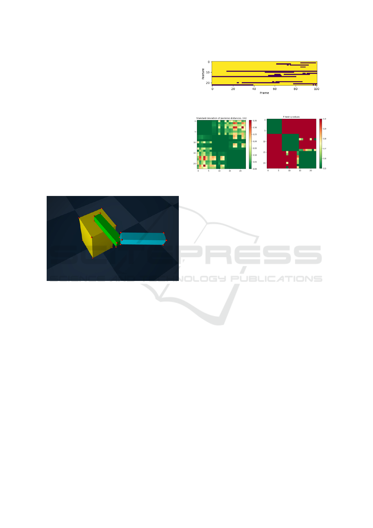
Figure 1: A 2-DoF arm on a base with keypoints (red dots)

simulated and tracked by MuJoCo over 100 steps.

We conducted an empirical veriﬁcation of the pro-

posed algorithm using a simulated robot arm with

two revolute joints in the MuJoCo physics engine

(Todorov et al., 2012) (see Fig. 1). To isolate the

algorithm’s performance from that of a feature track-

ing system, we directly extracted the 3D positions of

23 keypoints (marked as red dots) from the simulator.

These keypoints were placed at the vertices of three

rigid bodies in the scene – the base and two links.

MuJoCo’s RGB-D rendering capabilities were used

to determine the visibility of each keypoint from the

camera’s perspective at each time step. The robot arm

was actuated by applying constant torques to its joints

over a sequence of T = 100 control steps at a rate of

30 Hz, causing the links to complete approximately

one full rotation each. The resulting keypoint visibil-

ity matrix over time is shown in Fig. 2.

The rigid body identiﬁcation phase involved an-

alyzing the pairwise distances between all keypoint

pairs. Figure 3 shows the standard deviations of these

Figure 2: Visibility matrix of keypoints over time (yellow if

visible, dark brown if not).

Figure 3: Standard deviations of all pairwise distances (left)

and their associated q-values (right).

distances, along with the corresponding q-values ob-

tained from the F-test, after introducing measurement

noise of 1 mm. The results indicate that the F-test pro-

vides more uniform, robust, and discriminative dis-

similarity metrics compared to raw distance variance.

Dendrograms resulting from agglomerative clus-

tering with complete linkage using the two dissimilar-

ity metrics are shown in Figs. 4 and 5, respectively.

Both metrics do allow the successful identiﬁcation of

three well separated clusters that match exactly the

ground truth (the point indices at the horizontal axis),

but this process is much easier with the q-values than

with standard deviations. To produce ﬂat clustering

from the dendrogram, the latter needs to be cut at a

desired dissimilarity threshold. If standard deviations

are used, any threshold between slightly above σ

noise

and 0.19 would produce the correct number of clus-

ters (three). However, any threshold higher than that

would result in two clusters only, merging the points

for the two links. Thus, the correct threshold de-

pends on the range of motion of the rigid bodies in the

scene, making it difﬁcult to determine entirely from

collected data. In contrast, the q-values lie in a stan-

dard range, where points that satisfy the RBA end up

having dissimilarity around 0.5, and those that do not,

end up with dissimilarity very close to 1. This makes

it very easy to use a standard, domain-independent

threshold for producing ﬂat clustering, for example

0.8. Note also that the two points from the ﬁrst link

that are also somewhat close to some of the points

in the second link do not present any problem for

the clustering algorithm, as they are still closer to the

points in the ﬁrst link, so they are grouped with them,

and later the high dissimilarity of those other points

to the points in the second link prevent an incorrect

merger of the two clusters.

Observation-Based Inverse Kinematics for Visual Servo Control

205

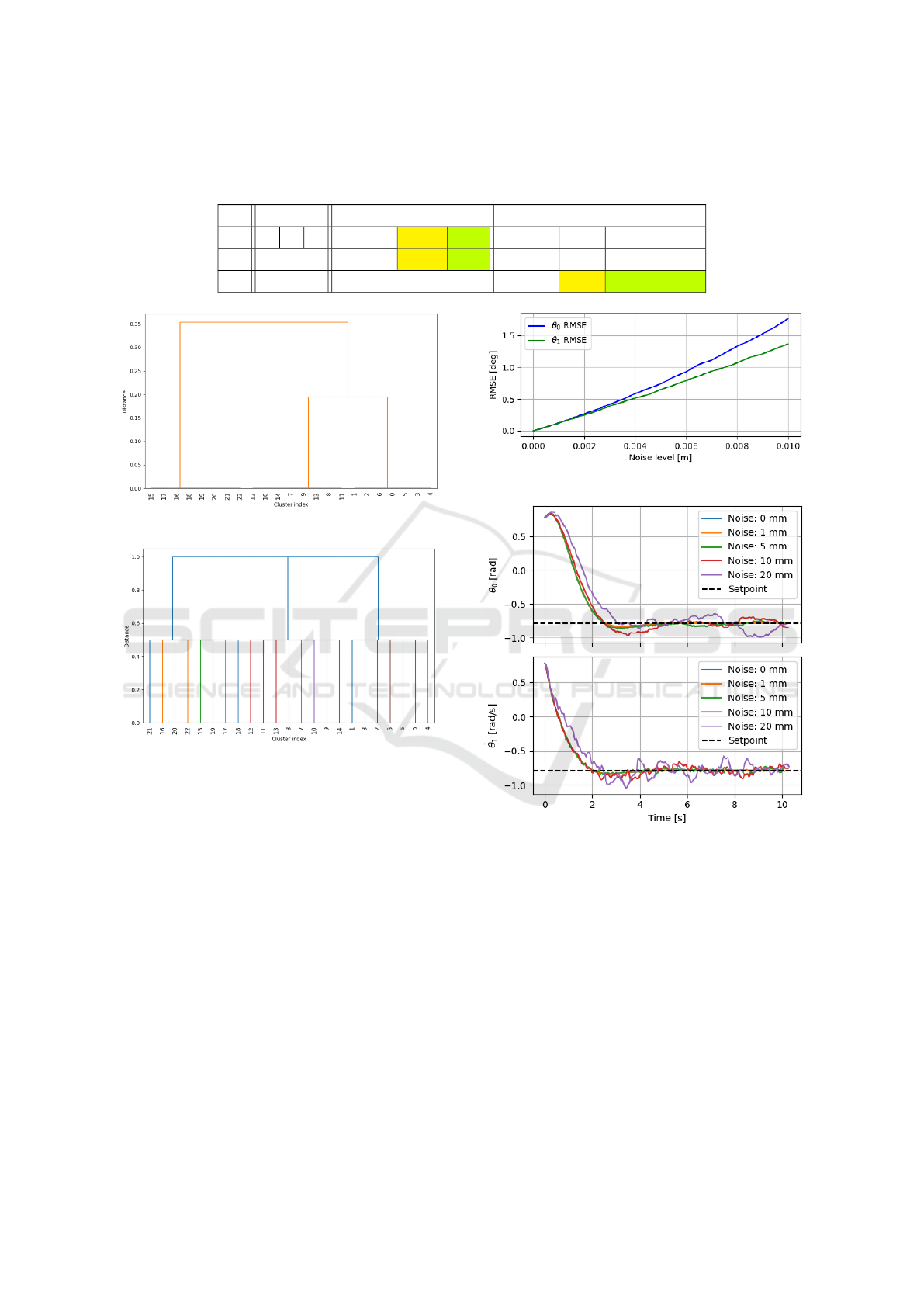
Table 1: Non-zero singular values of transform matrices between pairs of body frames. F

is the world frame and frames F

l = 1,2,3 are the frames attached to each of the three discovered rigid bodies. Each table entry shows singular values for the

translational, rotational, and center-of-rotation estimates for the relative RBTs. Colored cells indicate a single DoF.

- - - 2.9, 1.5 18.9 1.2 4.4, 3.1 19.6 10.2, 2.0, 0.4

2.9, 1.5 18.9 1.3 3.2, 2.8 19.6 10.1, 2.0, 0.4

6.0, 0.4 8.9 1.1

Figure 4: Dendrogram using standard deviations.

Figure 5: Dendrogram using q-values.

In the conﬁguration construction phase, the ranks

of the matrices T

and R

were computed for l =

0,1, 2 and m = l + 1,...,3, with the results summa-

rized in Table 1. Since no translational or rotational

degrees of freedom were detected between bodies 1

(the base) and 0 (the world frame), it can be concluded

that the base remains stationary. A single rotational

DoF was identiﬁed between bodies 1 and 2, indicating

that body 2 (the ﬁrst link) rotates relative to the base.

The presence of two translational DoFs between body

2 and both the world and base frames is explained by

the fact that body 2 rotates around the end of the ﬁrst

link, tracing an arc in a plane – kinematically equiva-

lent to 2D translation. This conﬁrms that the second

link is not directly connected to either the world or the

base via a joint. However, when analyzing the DoFs

of body 2 relative to the frame of body 1, the detec-

tion of a single rotational DoF conﬁrms the presence

of a revolute joint between the ﬁrst and second links.

Figure 6: RMSE of joint angle estimates.

Figure 7: Joint angles under PBVS using OBIK with vari-

ous levels of noise.

Because digital cameras have ﬁnite resolution,

a key question concerning the use of the proposed

method in practice is how quantization and other

measurement errors of the 3D positions of keypoints

would affect the accuracy of estimating the joint an-

gles of the mechanism. To investigate this empir-

ically, zero-mean Gaussian noise with various stan-

dard deviations was added to the keypoints’ 3D posi-

tions and the resulting estimates of joint angles were

compared with the true values reported by the simula-

tor. The root mean-squared error (RMSE) of the esti-

mates is shown in Fig. 6, averaged over 100 random-

number seeds. The error is less than 0.02

with noise-

ICINCO 2025 - 22nd International Conference on Informatics in Control, Automation and Robotics

206

free keypoint position measurements, and grows only

slightly faster than linearly with the level of keypoint

noise. For measurement error of 1 mm, joint angle es-

timation error on the order of 0.21

can be expected.

This suggests that the proposed method, although cer-

tainly not as accurate as dedicated angular encoders

on the joints, could be used for conﬁguration estima-

tion for the purposes of controlling the mechanism.

Ultimately, the most important question is how

measurement noise in the 3D positions of keypoints

affects the performance of a PBVS controller using

the proposed OBIK scheme for conﬁguration esti-

mation. To investigate this, a proportional-derivative

(PD) controller was applied to the 2-DOF mechanism

with the objective of moving it from initial conﬁgura-

tion (π/4, π/4) to goal conﬁguration (−π/4,−π/4).

The PD controllers for the two joints were indepen-

dent, with proportional gains K

= K

= 1 and

derivative gains K

= 1 and K

= 0.5 for links 1 and

2, respectively. The keypoint positions corresponding

to the goal conﬁguration were used as reference for

the OBIK method, meaning that the PBVS PD con-

troller was essentially trying to bring the estimated

joint conﬁguration to the origin, subject to measure-

ment noise in the keypoint positions at each control

step. Joint angle trajectories for the true angles of

both joints, as recorded by the physics engine, are

shown in Fig. 7 for several levels of measurement

noise. The controller reaches the setpoint reliably and

smoothly even for signiﬁcant noise, as high as 20 mm.

For noise on the order of 5 mm, which is already more

than what is typical of modern RGB-D cameras, even

in the depth dimension, the joint trajectories are vir-

tually indistinguishable from those corresponding to

when no measurement noise is present.

6 CONCLUSION AND FUTURE

WORK

We introduced a method for learning compact repre-

sentations of the conﬁguration of articulated mecha-

nisms from sequences of keypoint positions tracked

in camera images. The approach relies on analyz-

ing temporal variations in pairwise distances between

keypoints to statistically determine which ones satisfy

the RBA, thereby identifying groups that belong to

the same rigid body. By examining the rank of matri-

ces that capture the translational and rotational com-

ponents of estimated poses over time, the algorithm

infers the kinematic chain and the types of joints in it.

The constructed conﬁguration vector is as compact as

that of the actual joint positions, effectively function-

ing as a joint observer without requiring prior knowl-

edge of the mechanism’s kinematics or appearance.

In future work, we aim to apply this observer to

real-time monitoring and control of robotic systems

and other articulated mechanisms. We also plan to in-

vestigate its robustness to noise and keypoint tracking

errors, as in a real environment, changes in illumina-

tion and color, as well as lack of texture can lead to

false matches and imprecise measurements.

REFERENCES

Chaumette, F., Hutchinson, S., and Corke, P. (2016). Visual

servoing. Handbook of Robotics, pages 841–866.

Finn, C., Tan, X. Y., Duan, Y., Darrell, T., Levine, S., and

Abbeel, P. (2016). Deep spatial autoencoders for vi-

suomotor learning. In 2016 IEEE International Con-

ference on Robotics and Automation (ICRA), pages

512–519. IEEE.

Franklin, G. F., Powell, J. D., Emami-Naeini, A., and Pow-

ell, J. D. (2015). Feedback control of dynamic systems.

Prentice hall Upper Saddle River.

Jonschkowski, R. and Brock, O. (2015). Learning state rep-

resentations with robotic priors. Autonomous Robots,

39:407–428.

Kipf, T., Elsayed, G. F., Mahendran, A., Stone, A., Sabour,

S., Heigold, G., Jonschkowski, R., Dosovitskiy, A.,

and Greff, K. (2021). Conditional object-centric learn-

ing from video. arXiv preprint arXiv:2111.12594.

Lesort, T., D

ıaz-Rodr

ıguez, N., Goudou, J.-F., and Filliat,

D. (2018). State representation learning for control:

An overview. Neural Networks, 108:379–392.

Levine, S., Finn, C., Darrell, T., and Abbeel, P. (2016). End-

to-end training of deep visuomotor policies. Journal

of Machine Learning Research, 17:1–40.

Mojallizadeh, M. R., Brogliato, B., and Prieur, C. (2023).

Modeling and control of overhead cranes: A tutorial

overview and perspectives. Annual Reviews in Con-

trol, 56:100877.

Murtagh, F. and Contreras, P. (2012). Algorithms for hierar-

chical clustering: an overview. Wiley Interdisciplinary

Reviews: Data Mining, 2(1):86–97.

Nelles, O. (2020). Nonlinear dynamic system identiﬁcation.

Springer.

Siciliano, B. and Khatib, O. (2016). Springer handbook of

robotics. Springer International Publishing.

Szeliski, R. (2022). Computer vision: algorithms and ap-

plications. Springer Nature.

Todorov, E., Erez, T., and Tassa, Y. (2012). MuJoCo: A

physics engine for model-based control. In Interna-

tional Conference on Intelligent Robots and Systems,

pages 5026–5033. IEEE.

Umeyama, S. (1991). Least-squares estimation of transfor-

mation parameters between two point patterns. IEEE

Transactions on Pattern Analysis & Machine Intelli-

gence, 13(04):376–380.

Wahlstr

om, N., Sch

on, T. B., and Deisenroth, M. P. (2015).

Learning deep dynamical models from image pixels.

IFAC-PapersOnLine, 48(28):1059–1064.

Observation-Based Inverse Kinematics for Visual Servo Control

207