Using Linear Regression, Ridge Regression, Lasso Regression, and

Elastic Net Regression for Predicting Real Estate Price

Zhaorui Zeng

Aulin College, Northeast Forestry University, Harbin, Heilongjiang, China

Keywords: House Sale Price Prediction, Linear Regression, Ridge Regression, Lasso Regression, Elastic Net Regression.

Abstract: In the contemporary economic landscape, the real estate market wields significant influence, with housing

prices being a crucial factor affecting individuals, industries, and the overall economy. Fluctuations in housing

prices can impact people's living standards, investment decisions, and the stability of related industries. Thus,

accurately predicting housing sales prices is of utmost importance. This paper focuses on predicting housing

sales prices using linear regression, ridge regression, Lasso regression, and elastic net regression. The

principles and applications of the four regression models in price prediction are explored in detail. By

calculating evaluation metrics such as Mean Absolute Error (MAE), Mean Squared Error (MSE), and Root

Mean Squared Error (RMSE), the performance of each model is compared. The results show that linear

regression has an MAE of 0.092129, indicating normal performance. Ridge regression can address

multicollinearity issues with an MAE of 0.091513, but may overfit. Lasso regression and elastic net regression,

with MAEs of 0.087802 and 0.087756 respectively, can simplify models through feature selection, reducing

overfitting risks and improving the ability of generalization. Future research could expand data sources,

incorporate external variables, adopt advanced models, and utilize big data and deep learning technologies.

This research provides valuable references for real estate-related decision-making and promotes the

development of real estate price prediction research.

1 INTRODUCTION

In today’s modernized world and economic system,

the real estate market occupies a crucial position. On

the one hand, purchasing a house is one of the most

important issues for most people. As Çılgın, C. &

Gökçen, H. (2023) mentioned, owning a house is an

essential issue for both low and middle income people.

On the other hand, the real estate market plays a role

in any related industries, which indicates its function

in the world economy(Pai and Wang,2020). However,

the unexpected fluctuation of the real estate market

can bring several influences both economically and

socially. As Capellán, Sánchez Ollero, & Pozo(2021)

have mentioned, after the period of the 2008 housing

bubble burst, a decline of employment, unit sold, unit

built, and number of companies appeared. Thus,

forecasting real estate accurately is of great

importance for not only publicity but also for real

estate industries.

So far, the majority of scholars have been engaged

https://orcid.org/0009-0001-1458-2393

in exploring the current situation of machine learning

in real estate prediction. Singh, Sharma, and

Dubey(2020) utilized big data concepts and three

models –linear regression, random forest, and

gradient boosting –to forecast housing sale prices in

lowa. Their findings indicated that the gradient-

boosting model outperformed the others in terms of

forecasting accuracy. Pai and Wang (2020) employed

four machine learning models, such as least squares

support vector regression (LSSVR) and classification

and regression tree (CART), along with actual

transaction data from Taiwan. Among these, LSSVR

demonstrated excellent performance in predicting real

estate prices. AL - Gbury and Kurnaz (2020)

combined an artificial neural network and a grey wolf

optimizer to predict housing market prices, achieving

a high accuracy rate. These studies explored diverse

methods and models, offering valuable references for

real estate price prediction.

The paper aims to construct an efficient housing

sales price prediction model by applying three classic

Zeng, Z.

Using Linear Regression, Ridge Regression, Lasso Regression, and Elastic Net Regression for Predicting Real Estate Price.

DOI: 10.5220/0013700300004670

Paper published under CC license (CC BY-NC-ND 4.0)

In Proceedings of the 2nd International Conference on Data Science and Engineering (ICDSE 2025), pages 509-515

ISBN: 978-989-758-765-8

509

algorithms: linear regression, ridge regression, and

Lasso regression. Initially, it conducts a thorough

analysis of the housing price dataset, dealing with

outliers and missing values. Then, it explores the

algorithms' principles, model-building processes, and

their applications in price prediction. Finally, it

assesses the models' performance using multiple

indicators, compares different algorithms,

summarizes the research, and looks ahead to future

research directions.

2 METHODS AND MATERIALS

2.1 Data Collection

This study utilizes the Ames Housing dataset, which

was compiled by Dean De Cock for data science

education purposes

(https://www.kaggle.com/competitions/house-prices-

advanced-regression-techniques/overview).

The dataset is characterized by its

comprehensiveness, consisting of 79 explanatory

variables that describe almost every aspect of

residential homes in Ames, Iowa. These variables

cover a wide range of features, including the physical

characteristics of the houses (such as the height of the

basement ceiling, and number of bedrooms), location-

related factors (proximity to railroads), and various

other details about the property. In terms of the sample

size, the dataset contains a substantial amount of data,

providing a rich source for in-depth analysis.

Before being used in this research, the dataset

underwent preprocessing. The preprocessing steps

included handling missing data and dealing with

outliers. For missing data, different strategies were

employed based on the proportion of missing values in

each column. As for outliers, they were identified and

removed by examining the correlation between

variables such as `SalePrice` and others like

`OverallQual` and `GrLivArea`. This preprocessing

was carried out to enhance the quality of the dataset,

aiming to facilitate more accurate analysis and model

building.

2.2 Methods

In the research of predicting housing sales prices,

linear regression, ridge regression, Lasso

regression,and elastic net regression were applied.

Each algorithm has its unique concepts, principles,

and characteristics.

2.2.1 Linear Regression

Linear regression is a basic yet important algorithm.

Its concept is to establish a linear relationship

between the dependent variable (housing sales price)

and independent variables (such as house area, and

number of rooms). The principle is to use the least

squares method to find the optimal coefficients that

minimize the sum of the squared differences between

predicted and actual values. It is easy to interpret, as

the coefficients directly show the impact of each

factor on the price. However, it assumes a linear

relationship and may not perform well when the

relationship is complex or there are correlated

variables.

2.2.2 Ridge Regression

Ridge regression is an improvement over linear

regression. It addresses issues like multicollinearity

by adding a penalty term (L2 regularization) to the

loss function. The concept is to shrink the coefficients

towards zero while fitting the model. This helps in

stabilizing the model and improving its generalization

ability. In housing price prediction, it can handle

correlated features better than linear regression .

2.2.3 Lasso Regression

Lasso regression, using L1 regularization, has a

distinct feature - it can perform feature selection. The

concept is to minimize the sum of squared errors plus

a penalty on the absolute values of the coefficients.

This is very useful when dealing with a large number

of features in housing price prediction, as it simplifies

the model and improves interpretability. However, it

is more sensitive to the choice of the value compared

to ridge regression.

3 RESULTS

Table 1: The correlation between the explanatory variables

and Saleprice

YearRemodAdd 0.507101

YearBuilt 0.522897

TotRmsAbvGrd 0.533723

FullBath 0.560664

1stFlrSF 0.605852

TotalBsmtSF 0.613581

GarageArea 0.623431

GarageCars 0.640409

ICDSE 2025 - The International Conference on Data Science and Engineering

510

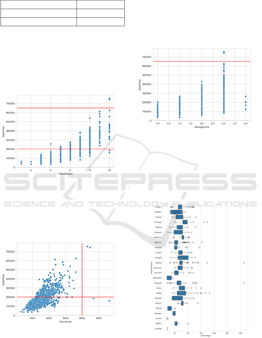
GrLivArea 0.708624

OverallQual 0.790982

SalePrice 1

The paper aims to find the correlation between the 74

explanatory variables and the house price and find out

that 10 of the variables-Fireplaces, YearRemodAdd,

YearBuilt, TotRmsAbvGrd, FullBath, 1stFlrSF,

TotalBsmtSF, GarageArea, GarageCars, GrLivArea,

and OverallQual- process large coefficient

association bigger than 0.5, which indicates the

correlations between this variable and the house price

is high (Table 1).

Figure 1: The correlation between House Sale Price and

Overall Quality Score (Picture credit : Original)

Figure 1 shows that the variable SalePrice has a

relatively low growth when OverallQual ranges from

2-4, however, it rises rapidly when OverallPrice

climbs to 8-10. Most data points cluster between

200000 and 650000, highlighting the relationship’s

significance for price prediction.

Figure 2: The Relationship between GrLivArea and

SalePrice(Picture credit : Original).

Figure 2 reveals the positively correlated

relationship between GrLivArea and SalePrice. When

GrLivArea is in the range of 0 - 1000, SalePrice

shows a slow growth. But when GrLivArea reaches

4000, SalePrice rises more significantly. Data points

mainly cluster in the lower-left area, where

GrLivArea is small (around 0 - 3000) and SalePrice is

relatively low (around 0 - 400000), indicating a large

number of such houses in the market.

Figure 3: The Relationship between House Sale Price and

the Number of Garage Cars(Picture credit : Original)

Figure 3 reveals a positive - correlation trend,

though not strictly linear. As GarageCars increase,

SalePrice generally rises. For different GarageCars

values like 0, 1, 2, and 3, there are multiple SalePrice

data points. A red horizontal line at y = 650000 shows

that high-price(above 650000) houses are less in

number.

Figure 4: The Distribution of Lot Frontage among different

Neighbourhoods(Picture credit : Original)

Using Linear Regression, Ridge Regression, Lasso Regression, and Elastic Net Regression for Predicting Real Estate Price

511

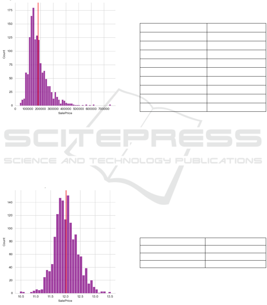
Figure 4 illustrates that as the values of

LotFrontage change, the spread and central - tendency

within each Neighbourhood differ. For different

Neighbourhoods, there are multiple LotFrontage data

points. The overall graph shows that extreme-value

(either very high or very low) LotFrontage in some

Neighbourhoods is less in number.

Figure 5: Distribution of House Sale Prices(Picture credit :

Original)

Figure 5 reveals a left-skewed distribution. The

data predominantly clusters on the left side, with most

values below the mean of around 200000. While there

exist some higher - value outliers extending to the

right, the majority of the data points contribute to the

concentration on the lower-price end, highlighting the

distinct left-leaning nature of the distribution.

Figure 6: Near-Normal Distribution of Log-Transformed

SalePrice Data(Picture credit : Original)

This barplot of SalePrice, after the np.log1p

transformation on the horizontal axis, reveals a near-

normal distribution (Figure 6). The data is

symmetrically clustered around the mean. The mean

of the data, indicated by the red vertical line, is

approximately at the value of around 12.0 on the log-

transformed scale.

Table 2: The Impact of Housing Features on Sale Price

Based on the Linear Regression Model

Id -0.000008

LotArea 0.000004

LotFrontage 0.000455

OverallCond 0.037583

OverallQual 0.037434

SaleCondition_AdjLand 0.181921

SaleCondition_Alloca 0.050358

SaleCondition_Family 0.000965

SaleCondition_Normal 0.075244

SaleCondition_Partial 0.068994

The coefficients in Table 2 result from defining

feature matrix X (excluding the SalePrice column)

and target variable y (the SalePrice column), splitting

the dataset into 70% training and 30% test sets, and

training a linear regression model.

These coefficients show each feature's influence

on SalePrice. A large absolute-value coefficient like

SaleCondition_AdjLand's (0.181921) implies a

stronger impact, while smaller coefficients suggest

weak correlations. This might be due to feature

irrelevance, multicollinearity, or data issues. Incorrect

train-test splits can cause underfitting or overfitting,

affecting model performance.

3.1 Linear Regression

Table 3: Performance Metrics of the Linear Model: MAE,

MSE, and RMSE

Quantity

MAE_linear 0.092129

MSE_linear 0.032784

RMSE_linear 0.181063

The evaluation metrics MAE (0.092129), MSE

(0.032784), and RMSE (0.181063) in Table 3 suggest

that the linear regression model has a relatively good

predictive performance. The presence of a certain

deviation between the predicted and actual values is

evident, as indicated by these metrics. This implies

that the model has room for improvement in

accurately predicting the target variable.

ICDSE 2025 - The International Conference on Data Science and Engineering

512

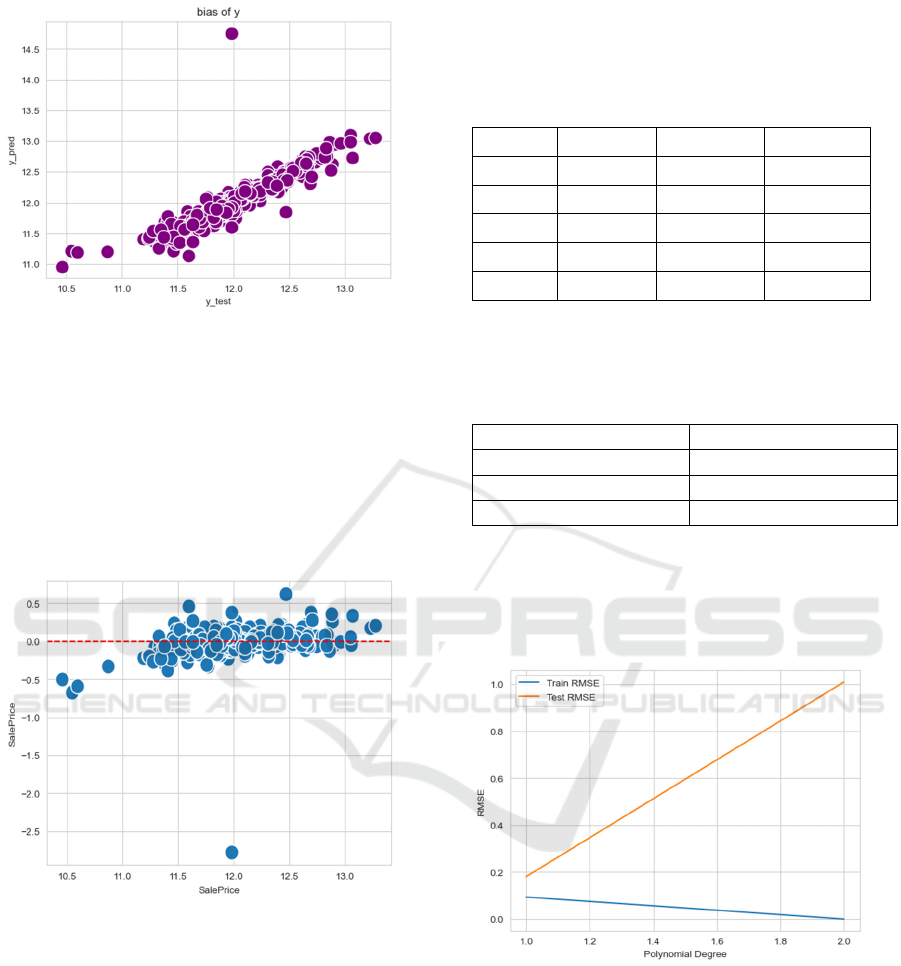
Figure 7: Correlation between Predicted and Actual House

Sale Prices(Picture credit : Original)

From Figure 7, it can be observed that the data

points are roughly distributed around a straight line

with x indicating the real value of the house sale price

and y revealing its predicted value, yet there are

discrete points. This indicates that there is a certain

correlation between the model's predicted values and

the actual values, but also a certain degree of

deviation.

Figure 8: Correlation between Predicted and the Difference

between Actual and Predicted Prices(Picture credit :

Original)

Figure 8 shows the relation between the real house

sell price and the difference value of the real and

predicted sale price, indicating that there still exist

discrete points.

Overall, the linear model is inappropriate for this

model with some of the discrete data.

3.2 Polynomial Regression model

Table 4: Variations between Actual and Forecasted Sale

Prices

Y_Test Y_Pred Y_Pred_2 Residuals

666 11.76758 13.16222 -1.39464

104 12.04061 11.96373 0.076878

528 11.36211 11.16076 0.201354

18 11.97667 12.19577 -0.2191

1151 11.91773 11.99526 -0.07753

Table 4 illustrates that there is a fluctuation between

the real house sale price and the predicted price.

Table 5:Performance Metrics of the Polynomial

Regression model: MAE, MSE, and RMSE

Metrics

MAE_Poly 0.309979

MASE_Poly 1.018768

RMSE_Poly 1.009240

Table 5 shows the MAE, MSE, and RMSE of this

model. With the value 0.309979 of MAE, it shows a

possibility of applying this model, however, the value

of MSE and RMSE are all above 1, which shows the

inaccuracy of the model in contrast.

Figure 9: Comparison of Training and Test Set RMSE with

Varying Polynomial Degrees from 1 to 2(Picture credit :

Original)

From Figure 9, although the training-set RMSE

experiences a slight decrease as the polynomial

degree increases from 1 to 2, the test-set RMSE rises

significantly. This indicates that increasing the

polynomial degree fails to improve the model's

predictive ability for new (test) data overall. Instead,

it may lead to overfitting, preventing the effective

reduction of errors.

Using Linear Regression, Ridge Regression, Lasso Regression, and Elastic Net Regression for Predicting Real Estate Price

513

3.3 Ridge Regression model

Table 6: Performance Metrics of the Ridge Regression

model: MAE, MSE, and RMSE

Metrics

MAE_Ridge 0.091513

MSE_Ridge 0.031576

RMSE_Ridge 0.177697

In Table 6, the evaluation metrics of the ridge

regression model are MAE (0.091513), MSE

(0.031576), and RMSE (0.177697), indicating a

relatively good predictive performance. These

metrics show that there is still some deviation

between the predicted and actual values. However,

compared to the linear regression model, the ridge

regression model has smaller values for MAE, MSE,

and RMSE, suggesting an improvement in accurately

predicting the target variable..

In the Ridge regression model, different features

are assigned varying weights. Features with positive

coefficients have a positive impact on the target

variable, while those with negative coefficients exert

a negative effect. Features with a coefficient of zero

indicate that they are not utilized in the model or

contribute minimally to the prediction. The

regularization mechanism in Ridge regression

effectively reduces the coefficients of certain features,

particularly those with redundancy or high correlation,

thereby enhancing the model's stability and

generalization ability. Overall, regularization helps

reduce overfitting and improves both the

interpretability and predictive accuracy of the model.

3.4 Lasso Regression model

Table 7: Performance Metrics of the Lasso Regression

model: MAE, MSE, and RMSE

Lasso Metrics

MAE_Lasso 0.087802

MSE_Lasso 0.031073

RMSE_Lasso 0.176275

The evaluation metrics for Lasso regression,

including MAE (0.087802), MSE (0.031073), and

RMSE (0.176275), indicate that the model

demonstrates reasonably good predictive

performance (Table 7). However, these metrics also

reveal some discrepancy between the predicted and

actual values, suggesting that there is still potential for

the model to improve in terms of accurately

forecasting the target variable.

Lasso regression results in a model with several

zero coefficients. This sparsity makes the model

simpler and more interpretable, reducing the risk of

overfitting and enhancing the model's generalization

ability.

3.5 Lasso Regression model

Table 8:Performance Metrics of the Elastic net Regression

model: MAE, MSE, and RMSE

Elastic Metrics

MAE_Elastic 0.087756

MSE_Elastic 0.029672

RMSE_Elastic 0.172257

The evaluation metrics MAE (0.087756), MSE

(0.029672), and RMSE (0.172257) for the Elastic

regression model indicate a reasonably good

predictive performance(Table 8). However, the

presence of some deviation between predicted and

actual values, as reflected by these metrics, suggests

that the model still has potential for improvement in

accurately forecasting the target variable.

Elastic net regression yields a model with several

zero coefficients. This sparsity makes the model

simpler and more interpretable, reducing the risk of

overfitting and enhancing the model's generalization

ability.

4 DISCUSSIONS

This study has yielded valuable results; however,

several limitations need to be addressed. Firstly, the

study uses a small and homogeneous sample, which

may limit the generalizability and reliability of the

findings, particularly across different regions or

groups. Secondly, the regression model assumes fixed

relationships, which fails to capture the complexity of

real-world dynamics. For example, external factors

such as policy changes or market non-linearity are not

fully considered, which may lead to prediction errors.

Thirdly, the study only considers a limited set of

features (e.g., price, location) and overlooks

potentially important factors such as surrounding

amenities or socio-economic conditions. Finally,

while the regression model is effective, it is sensitive

to outliers and noise, limiting its ability to handle

complex, nonlinear data patterns.

To improve the study, several suggestions can be

made. First, using diverse data sources and larger

samples would enhance the accuracy and

applicability of the findings. Second, incorporating

external factors such as policy changes and economic

trends would improve prediction accuracy, especially

in volatile markets like real estate. Third, more

ICDSE 2025 - The International Conference on Data Science and Engineering

514

advanced techniques (e.g., SVM, Random Forests)

should be employed to better handle non-linearities.

Finally, integrating Big Data and Deep Learning

technologies could improve model accuracy and

capture complex relationships within the data.

With improved data and computation, future

research can expand the study’s scope and incorporate

interdisciplinary methods for better prediction

capabilities.

5 CONCLUSION

This study focuses on predicting housing sale prices

using linear regression, ridge regression, ridge

regression, Lasso regression, and Elastic Net

regression. First, the housing data set from the Kaggle

platform was employed. After preprocessing the data

to handle missing values and outliers, the principles

and model–building processes of four regression

algorithms were explored. Then, these algorithms

were applied to construct prediction models and

multiple evaluation metrics like MAE, MSE, and

RMSE were used to assess the model’s performance.

The research findings indicate that different

regression models have varying different

performances. The linear regression model shows

mediocre predictive ability; ridge regression has the

potential for application but may suffer from

overfitting; Lasso regression and Elastic Net

regression can simplify the model through feature

selection, with relatively small error values, reducing

the risk of overfitting and enhancing generalization

ability.

Looking ahead, future studies can expand the data

sample size and source to improve accuracy and

applicability. Incorporating external variables such as

policy and economic trends, and adopting advanced

techniques like SVM and random forests can better

capture complex relationships. This research is

significant as it provides a reference for making

decisions related to real estate, which helps market

participants like home buyers, developers, and

investors make more informed choices.

REFERENCES

Al-Gbury, O., Kurnaz, S., 2020. Real estate price range

prediction using artificial neural network and grey wolf

optimizer. In IEEE 2020 4th International Symposium

on Multidisciplinary Studies and Innovative

Technologies (ISMSIT), Istanbul, Turkey, 2020.10.22-

2020.10.24.

Capellán, R. U., Luis Sánchez Ollero, J., Pozo, A. G., 2021.

The influence of the real estate investment trust in the

real estate sector on the Costa del Sol. European

Research on Management and Business Economics,

27(1).

Çılgın, C., Gökçen, H., 2023. Machine learning methods for

prediction real estate sales prices in Turkey. Revista de

La Construcción, 22(1), 163–177.

Dieudonné Tchuente;Serge Nyawa;. (2021). Real estate

price estimation in French cities using geocoding and

machine learning . Annals of Operations Research

Kaggle, n.d. House prices—Advanced regression

techniques. Retrieved from

https://www.kaggle.com/competitions/house-prices-

advanced-regression-techniques/overview

Kansal, M., Singh, P., Shukla, S., & Srivastava, S. (2023).

A Comparative Study of Machine Learning Models for

House Price Prediction and Analysis in Smart Cities.

In Communications in Computer and Information

Science (Vol. 1888 CCIS, pp. 168-184). Springer

Science and Business Media Deutschland GmbH.

Pai, P.F., Wang, W.C., 2020. Using machine learning

models and actual transaction data for predicting real

estate prices. Applied Sciences, 10(17), 5832.

Manjula, R; Jain, Shubham; Srivastava, Sharad; Rajiv Kher,

Pranav . (2017). Real estate value prediction using

multivariate regression models. IOP Conference Series:

Materials Science and Engineering, 263, 042098.

Nnadozie, L., Matthias, D., Bennett, E. O., 2022. A model

for real estate price prediction using multi-level

stacking ensemble technique. European Journal of

Computer Science and Information Technology, 10(3),

33–45.

Singh, A., Sharma, A., Dubey, G., 2020. Big data analytics

predicting real estate prices. International Journal of

System Assurance Engineering and Management, 11,

208–219.

Varma, Ayush; Sarma, Abhijit; Doshi, Sagar; Nair, Rohini .

(2018). [IEEE 2018 Second International Conference

on Inventive Communication and Computational

Technologies (ICICCT) - Coimbatore (2018.4.20-

2018.4.21)] 2018 Second International Conference on

Inventive Communication and Computational

Technologies (ICICCT) - House Price Prediction Using

Machine Learning and Neural Networks. , (), 1936–

1939. doi:10.1109/ICICCT.2018.8473231

Using Linear Regression, Ridge Regression, Lasso Regression, and Elastic Net Regression for Predicting Real Estate Price

515