
Time Series Analysis and Prediction of Future Commodities Prices
with SARIMA
Siyou Yao
a
Finance Management School, Shanghai University of International Business and Economics, Shanghai, China
Keywords: SARIMA, Future Commodities Prices, Forecast, Transaction.
Abstract: Commodities are one of the most important investing targets in the world. Forecasting the prices of
commodities precisely helps investors and corporations make reasonable transactions. This paper is based on
the prices of Brent oil, wheat, and aluminum and predicts the future prices of commodities in the energy
industry, the manufacturing industry, and the agricultural products industry. The results show that the
Seasonal Autoregressive Integrated Moving Average (SARIMA) model has a relatively excellent ability to
predict the future movements of the commodities prices. The prediction shows that all the commodities prices
will experience a decline in the next 10 months. However, the predictions are not exactly the same as the
actual movements. The fluctuation extent of the predictions is much smaller. Therefore, the SARIMA model
can help investors establish a broad idea of the future trend of the commodities prices, but it cannot help
investors do ultrashort-term trading. If the investors only focus on the trend during a longer period and ignore
making profits with the short-term fluctuations, the SARIMA model is suitable for them. In the end, this paper
suggests investors combine the fundamental analysis with the forecasting results generated by the SARIMA
model to make trading decisions.
1 INTRODUCTION
Commodities are raw materials and resources that are
normalized, tradable, and low value-added. They also
have a large volume in nature. Commodities are often
divided into three categories (Zhou, Song, & Ren,
2022): energy commodities, metal commodities, and
agricultural products commodities. As the upstream
raw material for many products, commodities have
important impacts on the development of the world
economy. Metals are unreplaceable resources and are
widely used in the manufacturing industry, oil and gas
are nonrenewable strategic resources that are the
objects of competition between the world's major
powers and leading economies, and agricultural
products are important in the food industry and can
help stabilize society (Guo, 2023). As the indicator of
the international situation, the movement of the prices
of commodities often represents macroeconomic
changes in the world, the change in supply and
demand, and the change in the market. Last but not
least, commodities can be traded by futures and
options. Investors can use commodities to earn
a
https://orcid.org/0009-0006-2814-2272
revenues and hedge risks. Therefore, it is meaningful
to predict the future movement of the prices of
commodities. It can help investors, companies, and
countries to make more reasonable decisions.
In 2021, Wanjuki et al. researched the Seasonal
Autoregressive Integrated Moving Average
(SARIMA)’s ability to forecast the price index of
food and beverages in Kenya (Wanjuki, Wagala, &
Muriithi, 2021). After comparing all the models with
different parameters, it turned out that SARIMA (1, 1,
1) (0, 1, 1)12 was the best fit for the data in the study.
In 2022, Li et al. applied the ARIMA model to gold
prices and gave investing suggestions based on the
forecasting results (Li, 2022). The study encouraged
investors to combine international situations with the
results. In 2023, ARIMA and SARIMA’s ability to
predict future crude oil prices were compared by
Ariyanti, and it turned out that both models were
excellent in forecasting (Ariyanti & Yusnitasari,
2023), which meant ARIMA and SARIMA models
were suitable for time series analysis of crude oil
prices. Gasper et al. conducted a study on forecasting
crude oil prices in Tanzania using the ARIMA model
Yao, S.
Time Ser ies Analysis and Prediction of Future Commodities Prices with SARIMA.
DOI: 10.5220/0013699500004670
Paper published under CC license (CC BY-NC-ND 4.0)
In Proceedings of the 2nd International Conference on Data Science and Engineering (ICDSE 2025), pages 467-475
ISBN: 978-989-758-765-8
Proceedings Copyright © 2025 by SCITEPRESS – Science and Technology Publications, Lda.
467

(Gasper & Mbwambo, 2023). This study found out
that even under the serious fluctuation caused by the
conflict in Ukraine and the coronavirus outbreak, the
ARIMA model could still capture the potential
movement in crude oil prices. In 2024, Guzman
affirmed ARIMA’s ability to predict future corn
prices in Mexico (Guzma, 2024). This research also
emphasized the importance of forecasting future
prices of agricultural products by pointing out that
future corn prices would influence farmers' interests
and sustainable agricultural development. Bagrecha
et al. used the ARIMA model to forecast silver prices
in India. However, the results only explained 26% of
the observed silver price changes. It suggested that
the ARIMA model was too simple for silver price
prediction and that more factors should be taken into
consideration (Bagrecha et al., 2024). In 2025, Ojha
et al. utilized the SARIMA model to predict global
wheat prices (Ojha & Karki, 2025). They pointed out
its importance in helping investors and countries
make reasonable strategic decisions. However, the
study claimed that the prediction is only suitable for
short-term analysis, and many external factors are not
considered. The results may not fit other commodities
and periods.
This paper aims to improve the ability to predict
the future prices of different commodities with the
SARIMA model, hoping to expand from the price
prediction of the commodity to the prediction of the
future development trend of the industry
corresponding to that commodity, and finally explore
the changes in industries and changes in the world
economy. This study first searches the prices of the
commodities in each of the three categories
mentioned above. Based on the different
characteristics of all the commodities in each
category, this study finally chooses aluminum in
metals, wheat in agricultural products, and Brent oil
in energy as the data to be researched. This paper first
applies pre-processing procedures to the data and then
uses the SARIMA model to fit the data and make
forecasts of future data in the next 10 months. The
differences between the future data and the actual
data are compared to evaluate the ability of the
SARIMA model. Conclusions are reached based on
the results and international events during the
research period.
2 DATASETS
2.1 Data Collection and Description
This paper extracts the datasets from Kaggle, and the
original datasets are extracted from Alpha Vantage
API using Python. The dataset contains monthly
historical prices of 10 different commodities from
January 1990 to March 2023. Prices are reported in
USD per unit of measurement for each commodity.
The prices of aluminum, wheat, and Brent crude oil
were selected in the study.
Crude oil is one of the most important energies in
the world. It can represent the energy industry. This
paper selects the price of the Brent crude oil which is
a blended crude stream produced in the North Sea
region. This is because Brent crude oil is one of the
most important crude oil pricing benchmarks in the
world. It is widely used in international oil price
quotation and contract settlement, and it serves as a
marker for pricing a number of other crude streams.
Compared with OPEC and WTI prices, the price of
Brent crude oil is more comprehensive and
transparent, because it is not affected by the US
domestic factors and the political factors of the
Organization of the Petroleum Exporting Countries
(OPEC).
Aluminum is widely used in aerospace,
automotive, construction, packaging, and many other
manufacturing and industrial sectors. It can represent
the manufacturing industry. The price movement of
aluminum directly reflects the economic performance
and industry cycles. Compared to gold and silver,
aluminum is less used as a precious metal and
investment target. Therefore, its price volatility is
usually less influenced by macroeconomic
uncertainty and safe-haven demand, which makes it
more appealing data in this study.
Wheat is one of the world's leading food crops. It
is widely used in food production and is important in
global agricultural trade. It can represent the
agricultural industry. Compared with other
agricultural products, wheat has a wider application.
For example, it can be processed into bread and beer.
2.2 Data Pre-processing
Since the characteristics of the prices of different
commodities are similar, the data pre-processing is
the same. Therefore, this paper will only focus on the
overall procedure in this part.
First of all, this paper generates the time series
plots of the prices of three commodities, the results
are shown in Figures 1, 3, and 5. From the plots, it
should be decided whether the prices of the three
commodities are stationary. This paper then applies
the log transformation to the data to make them
stationary. This paper also uses STL decomposition
to detect the characteristics of the data. The results are
shown in Figures 2, 4, and 6. From the four plots
ICDSE 2025 - The International Conference on Data Science and Engineering
468
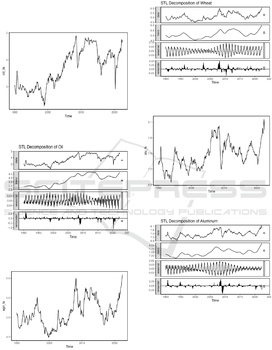
generated by the STL decomposition, the seasonality,
trend, and volatility can be checked. Then, it can be
decided which model to use.
Figure 1: The Time Series Plot of the Brent Oil Prices after
Log Transformation. (Picture credit: Original)
Figure 2: The STL Decomposition on Brent Oil Prices.
(Picture credit: Original)
Figure 3: The Time Series Plot of the Wheat Prices after
Log Transformation. (Picture credit: Original)
Figure 4: The STL Decomposition on Wheat Prices.
(Picture credit: Original)
Figure 5: The Time Series Plot of the Aluminum Prices
after Log Transformation. (Picture credit: Original)
Figure 6: The STL Decomposition on Alunimun Prices.
(Picture credit: Original)
From the time series plot of the Brent oil prices,
wheat prices, and aluminum prices, it is obvious that
the data is not stationary even after the log
transformation. It means that the data need a
differencing process. According to the decomposition,
all the data show a slightly upward trend and
seasonality. The remainders show that the
Time Series Analysis and Prediction of Future Commodities Prices with SARIMA
469
characteristics of the data have been nearly fully
extracted by the trend and seasonality.
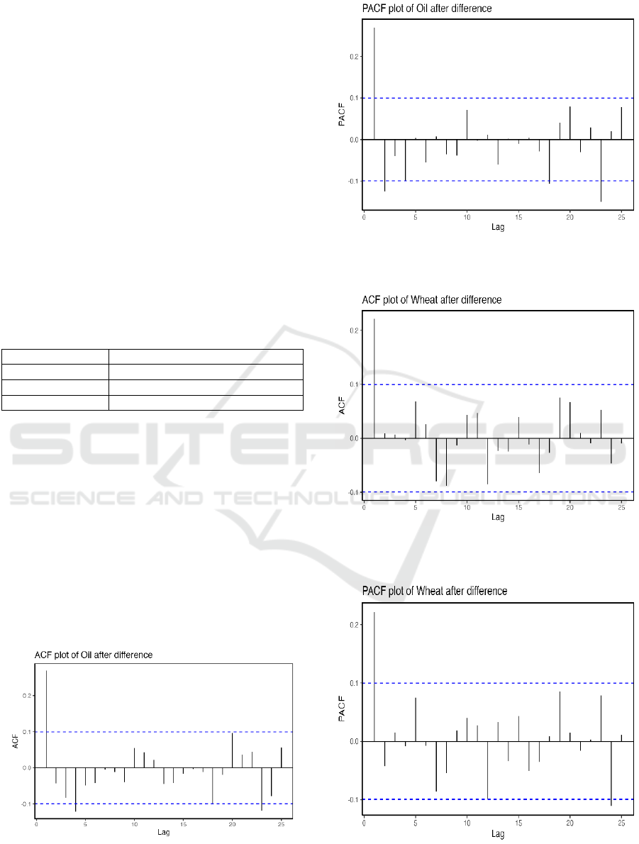
Therefore, this paper generates the ACF plot and
the PACF plot to further check whether the data are
stationary. The results show that the autocorrelation
of all three datasets has a downward trend as the lag
increases. In addition, the PACF values of the data are
extremely large when the lag equals one. All in all, it
means that the data are not stationary even after the
log transformation. The data may need differencing.
To further ensure whether the data need
differencing, this study also utilizes the Augmented
Dickey-Fuller unit root test as the stationary test. The
test can identify stationary data and judge whether the
data needs differencing. If the p-value is bigger than
0.05, the test will reject the null hypothesis that the
time series data is not stationary and has a unit root.
The results are shown in Table 1.
Table 1: The Results of ADF Tests on Commodities Before
Differencing.
Commodity
ADF test before differencing
Oil
p-value = 0.3696
Wheat
p-value = 0.4663
Aluminum
p-value = 0.03145
From Table 1, the p-values of the Brent oil prices,
the wheat prices, and the aluminum prices are 0.3696,
0.4663, and 0.03145 respectively. It can be seen that
the p-values of the Brent oil prices and the wheat
prices are much larger than 0.05, while the p-value of
the aluminum prices is less than 0.05. Combined with
all the results reached above, this research conducts a
first-order differencing to all the data.
After the differencing, both the ACF and PACF
plots and the ADF test are utilized again to decide
whether the data needs more processing procedures.
The results are shown in Figures 7, 8, 9, 10, 11, and
12 and Table 2.
Figure 7: The ACF Plot of the Brent Oil Prices after
Differencing. (Picture credit: Original)
Figure 8: The PACF Plot of the Brent Oil Prices after
Differencing. (Picture credit: Original)
Figure 9: The ACF Plot of the Wheat Prices after
Differencing. (Picture credit: Original)
Figure 10: The PACF Plot of the Wheat Prices after
Differencing. (Picture credit: Original)
ICDSE 2025 - The International Conference on Data Science and Engineering
470
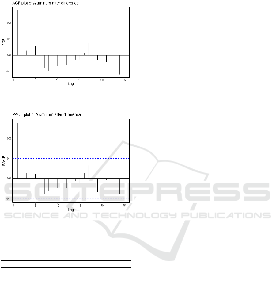
Figure 11: The ACF Plot of the Aluminum Prices after
Differencing. (Picture credit: Original)
Figure 12: The PACF Plot of the Aluminum Prices after
Differencing. (Picture credit: Original)
Table 2: The Results of ADF Tests on Commodities after
Differencing.
Commodity
ADF test after differencing
Oil
p-value = 0.01
Wheat
p-value = 0.01
Aluminum
p-value = 0.01
Based on the ACF and PACF plots, it can be
detected that the ACF and PACF are the largest when
the lag equals one. As the lag increases, the ACF and
PACF decrease immediately to zero. It means that the
AR (1) model is suitable for all the data and all the
data are stationary now.
After the differencing, all the data pass the ADF
test. Therefore, all the data are certainly stationary.
2.3 Model
This paper uses the decomposition method, plotting,
and the SARIMA model for analysis and prediction.
The ARIMA (Autoregressive Integrated Moving
Average) model developed by Box and Jenkins is one
of the most basic and important models in time series
analysis. The SARIMA model adds seasonal factors
to the original ARIMA model. It is more suitable for
the data with high seasonality. The SARIMA model
can be expressed as (1):
ARIMA
(
p, d, q
)(
P, D, Q
)
m
(
1
)
the parameter p represents the order of the AR
(Autoregressive) component, which captures the
linear relationship between the current observation
and its previous observations. The parameter d means
subtracting the previous observation from the current
one d times to remove trends and make the series
stationary. The parameter q is the order of the MA
(Moving Average) component, which shows the
relationship between an observation and a residual
error from a moving average model applied to lagged
observations. On the other hand, the parameters P, D,
and Q have similar functions with p, d, and q, but they
are applied to the seasonal components. m is the
seasonal period.
The auto.arima function is applied to the data to
make the computer automatically select the best
model. However, the model should be further selected
based on the evaluation indicators, and the PACF
plots.
2.4 Evaluation
This paper focuses on Root Mean Squared Error
(RMSE), Akaike Information Criterion (AIC), and
Bayesian Information Criterion (BIC) as the
evaluation indicators for prediction. RMSE calculates
the average of the squares of the differences between
predicted and actual values, which helps measure the
model error. AIC is an indicator used to select the
model, and it balances the goodness of fit and
complexity of the model. BIC punishes more on the
complex model compared to AIC. It tends to choose
a simpler model.
This paper also focuses on the fitting ability of the
SARIMA model. Considering that the SARIMA
model has 6 parameters, this study will use an
adjusted R square as the evaluation indicator. The
adjusted R square can help avoid the situation that the
R square will increase freely. as the complexity of the
model increases. It can protect the model from
overfitting.
Time Series Analysis and Prediction of Future Commodities Prices with SARIMA
471
3 EXPERIMENT RESULTS AND
ANALYSIS
Sometimes, the auto.arima function cannot select the
best model because it only focuses on minimizing the
AIC and BIC values but not the RMSE values.
Additionally, the auto.arima function may not try
every combination of the six parameters. This paper
further selected the model based on the values of AIC,
BIC, and RMSE. The smaller the values of these
indicators, the better the model is. Each combination
of the six parameters is tested. The parameters p, P, q,
and Q take the values 0, 1, and 2, the parameter d
constantly equals 1, and the parameter D takes the
values of 0 and 1. The results are shown in Tables 3,
4, and 5.
Table 3: SARIMA Models on Brent Oil Prices with
Different Parameters.
(p, d, q)
(P, D, Q)
AIC
BIC
RMSE
(0,1,1)
(0,0,1)
-696.566
-684.683
0.0978
(0,1,1)
(1,0,0)
-696.489
-684.606
0.0978
(0,1,1)
(0,0,2)
-696.636
-680.792
0.0974
(0,1,1)
(2,0,0)
-696.365
-680.521
0.0975
(0,1,1)
(1,0,1)
-696.195
-680.351
0.0975
(1,1,2)
(1,0,0)
-697.365
-677.56
0.0971
(0,1,1)
(2,0,2)
-698.882
-675.116
0.0947
Table 4: SARIMA Models on Aluminum Prices with
Different Parameters.
(p, d, q)
(P, D, Q)
AIC
BIC
RMSE
(1,1,0)
(2,0,0)
-1268.17
-1252.33
0.0466
(0,1,1)
(0,0,2)
-1268.16
-1252.32
0.0466
(0,1,1)
(2,0,0)
-1267.98
-1252.14
0.0466
(0,1,1)
(0,0,1)
-1263.53
-1251.65
0.0471
(2,1,0)
(0,0,2)
-1266.91
-1247.1
0.0466
(0,1,1)
(1,0,0)
-1262.94
-1251.06
0.0471
(1,1,1)
(0,0,2)
-1266.89
-1247.09
0.0466
Table 5: SARIMA Models on Wheat Prices with Different
Parameters.
(p, d, q)
(P, D,
Q)
AIC
BIC
RMSE
(0,1,1)
(0,0,1)
-1020.07
-1008.19
0.064
(0,1,1)
(1,0,0)
-1019.31
-1007.43
0.0645
(1,1,0)
(0,0,1)
-1019.14
-1007.26
0.0645
(1,1,0)
(1,0,0)
-1018.46
-1006.58
0.0645
(0,1,1)
(0,0,2)
-1020.44
-1004.6
0.0642
(2,1,1)
(0,0,1)
-1022.3
-1002.49
0.0638
(0,
1,1)
(1,
0,2)
-
1021.01
-
1001.21
0.0
638
Finally, the best model is selected for each
commodity. For Brent oil, the best model is SARIMA
(0, 1, 1) (2, 0, 2), and the AIC value equals -698.882,
the BIC value equals -675.116 and the RMSE value
equals 0.094708. For Aluminum, the best model is
SARIMA (1, 1, 0) (2, 0, 0), and the AIC value equals
-1268.17, the BIC value equals -1252.33 and the
RMSE value equals 0.046628. For the wheat, the best
model is SARIMA (2, 1, 1) (0, 0, 1), and the AIC
value equals -1022.3, the BIC value equals -1002.49
and the RMSE value equals 0.063838.
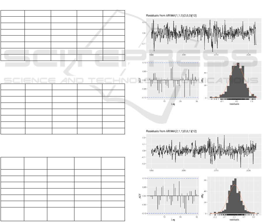
This paper uses the checkresiduals function to
check whether the residuals of the model are
consistent with the white noise. If the residuals are not
independent and are not consistent with normal
distribution, the model selected may not be suitable
for the study. Autocorrelation and time series plots of
the residuals can be tested by the ACF plot and the
Ljung-Box test in the function. The results of
aluminum prices, wheat prices, and Brent oil prices
are shown in Figures 13, 14, and 15 respectively. The
results of the Ljung-Box tests are shown in Table 6.
Figure 13: The Residuals Check on the SARIMA Model of
Aluminum Prices. (Picture credit: Original)
Figure 14: The Residuals Check on the SARIMA Model of
Wheat Prices. (Picture credit: Original)
ICDSE 2025 - The International Conference on Data Science and Engineering
472
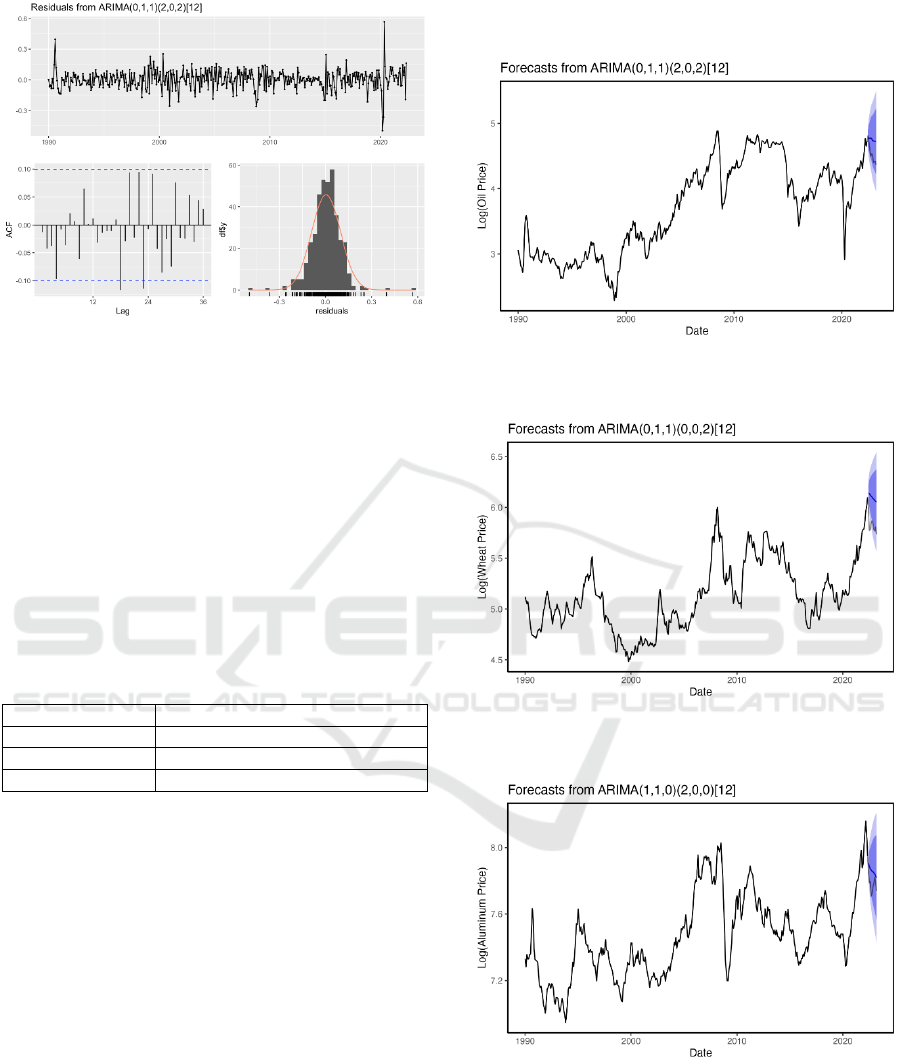
Figure 15: The Residuals Check on the SARIMA Model of
Brent Oil Prices. (Picture credit: Original)
From the residuals plots, the residuals have
random fluctuations around zero mean, which means
that the model has a good fit. According to the ACF
plots of the SARIMA models of the data, the
autocorrelation values for most lags are within
confidence intervals, which means the residuals of the
SARIMA model are consistent with white noise.
According to the histogram, the residuals are
consistent with normal distribution. All the data pass
the residuals check.
Table 6: Ljung-Box Test of Residuals of All SARIMA
Models
Commodity
Ljung-Box test of Residuals
Oil
p-value = 0.08311
Wheat
p-value = 0.6398
Aluminum
p-value = 0.5808
All the p-values of the Ljung-Box test of residuals
are larger than 0.05. This indicates that there is no
significant autocorrelation in the residuals and that
the residuals are white noise. The model has captured
all the autocorrelation structures in the data, and the
residuals do not contain any systematic patterns,
which is the same as the conclusion from the ACF
plots above.
In the forecasting part, this research generates the
future movement of the prices of three commodities
in the next 10 months. The confidence intervals are
also generated. Finally, the real movement of the
prices is shown in the same picture as the predicted
movement to help offer some meaningful investing
suggestions. In the forecasting plots below, the
translucent black line indicates the historical data, the
blue line is the predicted mean, and the light blue and
dark blue areas indicate 80% and 95% confidence
intervals, respectively. The results are shown in
Figures 16, 17, and 18.
Figure 16: Brent Oil Prices Prediction Compared with
Actual Values. (Picture credit: Original)
Figure 17: Wheat Prices Prediction Compared with Actual
Values. (Picture credit: Original)
Figure 18: Aluminum Prices Prediction Compared with
Actual Values. (Picture credit: Original)
From the three plots above, the Brent oil price will
slightly go down in the next 10 months, and the prices
of aluminum and wheat will experience a sharp
decline in the next 10 months.
Time Series Analysis and Prediction of Future Commodities Prices with SARIMA
473
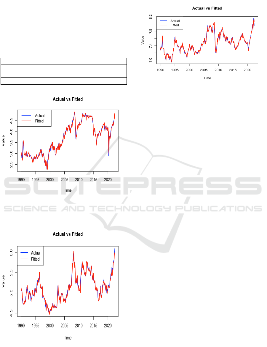
In the fitting part, this study calculated the
adjusted R square to find out the fitting ability of the
model. The results of the adjusted R square are shown
in Table 7. The plots of the actual values and the fitted
values of three commodities are shown in Figures 19,
20, and 21.
Table 7: Adjusted R2.
Commodity
Adjusted R square
Oil
0.9799
Wheat
0.9632
Aluminum
0.9631
Figure 19: Fit Chart of Brent Oil Prices. (Picture credit:
Original)
Figure 20: Fit Chart of Wheat Prices. (Picture credit:
Original)
Figure 21: Fit Chart of Aluminum Prices. (Picture credit:
Original)
It turns out that three SARIMA models fit well
with the data. The values of the adjusted R square of
Brent oil, wheat, and aluminum are 0.9799, 0.9632,
and 0.9631 respectively.
Although the forecasting declines are not that
serious compared with the actual fluctuation of the
prices of the three commodities. The trends of the
future movement are clear enough for investors to
decide their next transaction.
The results from this study are not enough because
the forecasting is not precise enough for investors to
decide when to buy and when to sell. Therefore,
investors need to combine some other factors such as
some international events in politics and some news
to make a reasonable transaction. In this study,
considering the decline in demand and supply caused
by the conflict in Ukraine, extreme weather, and
geopolitical conflicts (Ji, 2023), the commodities
prices are more likely to experience a downward
trend (Liu, 2022). Therefore, short selling for all
commodities mentioned above is a good choice.
In addition, some characteristics of the data may
not be extracted completely. To make a more precise
prediction and to help investors invest only by time
series analysis, a more complex model or a combined
model needs to be applied.
4 CONCLUSIONS
From the research, this paper discovers that the
SARIMA model has a relatively excellent ability to
predict the future prices of commodities. For
aluminum, the prediction shows that its price will go
down and the confidence interval is large, which
means it is not wise to buy aluminum in May 2022
and the price of aluminum can fluctuate a lot. For
wheat, the prediction also shows a decrease in price
ICDSE 2025 - The International Conference on Data Science and Engineering
474

but the confidence interval is smaller, which means it
is not wise to buy wheat in May 2022, and the
fluctuation in wheat price will be smoother. For oil,
the trend of the prediction is not obvious because
there is only a slight decrease, and the confidence
interval is also smaller, which means it may not be
wise to buy oil in May 2022, and the price of the oil
will not fluctuate a lot in the next 10 months. From
the actual values, it turns out that the real movement
of the prices of aluminum and wheat is almost the
same as the prediction. On the contrary, the difference
between the prediction of the Brent oil prices and the
actual values is not neglectable. It indicates that the
SARIMA model has a better forecasting ability in the
agricultural industry and the manufacturing industry
than in the energy industry. Overall, if investors make
decisions based on the prediction, they will not lose
money but can even earn some money by short selling.
However, the prediction of the future prices of three
commodities is not extremely precise, which means
people are not able to do short-term trading and
ultrashort-term trading because they will lose some
opportunities to make profits. In the future, more
complex models that can include more samples and
some other factors such as international events,
fundamental analysis, and investors’ minds should be
considered. In addition, the SARIMA model can be
combined with other methods, such as BNPP to
further make a more precise prediction.
REFERENCES
Ariyanti, V. P., & Yusnitasari, T. (2023). Comparison of
ARIMA and SARIMA for forecasting crude oil prices.
Jurnal RESTI (Rekayasa Sistem dan Teknologi
Informasi, 7(2), 405-413.
Bagrecha, C., Singh, K., Sharma, G., & Saranya, P. B.
(2024). Forecasting silver prices: A univariate ARIMA
approach and a proposed model for future direction.
Mineral Economics, 1-11.
Gasper, L., & Mbwambo, H. (2023). Forecasting crude oil
prices by using ARIMA model: Evidence from
Tanzania.
Guo, M. (2023). A study on the impact of international
commodity price volatility on China's macroeconomy
(Doctoral dissertation, Sichuan University).
Guzma, L. (2024). Application of ARIMA model to
forecast corn prices in Mexico. Scientia et PRAXIS,
4(08), 63-95.
Ji, J. (2023). Commodity price trends in 2022 and outlook
for 2023. Contemporary Petroleum and Petrochemicals,
31(4), 1-3.
Li, C. S. (2022). Forecasting gold price changes in China
using time series. Industrial Innovation Research, 23,
81-83.
Liu, N. (2022). Analysis of major commodity price trends
since 2022. China Price Regulation and Antimonopoly,
9, 68-69.
Ojha, S., & Karki, L. B. (2025). Forecasting global wheat
price in the context of changing climate and market
dynamics: An application of SARIMA modeling
technique.
Wanjuki, T. M., Wagala, A., & Muriithi, D. K. (2021).
Forecasting commodity price index of food and
beverages in Kenya using seasonal autoregressive
integrated moving average (SARIMA) models.
European Journal of Mathematics and Statistics, 2(6),
50-63.
Zhou, Z., Song, Z., & Ren, T. (2022). Predicting China's
CPI by scanner big data. arXiv preprint
arXiv:2211.16641.
Time Series Analysis and Prediction of Future Commodities Prices with SARIMA
475
