Predicting Apple Inc. Stock Prices Using Machine Learning
Techniques
Yuanchen Wang
a
Department of Sciences, Shanghai University, Shanghai, China
Keywords: Machine Learning, Future of Stocks, Combined Models, Prediction.
Abstract: The accurate prediction of financial asset prices is essential to the finance industry, where decisions rely
heavily on future price forecasting. Using machine learning methods to forecast future closing values of
financial assets is examined in this study. To improve resilience and forecast accuracy, this research integrates
individual models like as Random Forest, Linear Regression, and Extreme Gradient Boosting (XGBoost) with
ensemble methods like voting classifiers. Metrics like Mean Squared Error (MSE), Mean Absolute Error
(MAE), and 𝑅

Score are employed to assess the models' effectiveness after they have been trained on
historical data. Additionally, in order to produce a more reliable forecast, this study proposes a combined
model technique that combines forecasts from several models. This paper aims to explore and optimize the
combined application of different machine learning models to provide a more reliable decision support tool
for financial market analysis, and ultimately provide investors and financial analysts with more forward-
looking market insights.
1 INTRODUCTION
In today's global financial markets, there are many
ways to predict financial time series. These methods
exist alongside the goods and labor markets (Rani &
Sikka, 2012). Stock price prediction is a trendy issue
for investors and scholars. However, it is really hard
to do. To predict the stock market, people use all
kinds of methods and data sources. Gunduz et al.
focused on integrating sentiment analysis from social
media with traditional financial indicators,
demonstrating that incorporating external data
sources could improve prediction performance.
(Gunduz et al., 2017). Chou et al. used support vector
machines (SVM) to model the relationship between
historical stock prices and future trends, achieving
robust results in volatile markets (Chou et al., 2014).
Convolutional neural networks (CNN) and long
short-term memory (LSTM) networks were coupled
in a deep learning framework by Long et al. to
efficiently capture temporal and spatial relationships
in stock data (Long et al., 2019). The most popular
approach is to build a model that uses past behavior
to predict future price trends. People also use
historical market data to forecast future prices (Kim
a
https://orcid.org/0009-0001-1807-8995
& Han, 2000). Wei et al. studied the application of
SVM for predicting stock market direction of motion,
highlighting the model’s efficacy in handling
complicated nonlinear data (Wei et al.,2005)
Over time, more traditional prediction methods
have been developed. These consist of logistic
regression, random forests, statistical techniques,
linear and quadratic discriminant analysis, and
evolutionary computation algorithms. (Hu et al.,
2019).
A collection of random financial variable values
over time is known as a financial time series.
According to Rani and Sikka, time series clustering is
a crucial concept in data mining (Rani & Sikka,
2012). Clustering enables us to forecast the future
values of time series and comprehend how they are
created. But in the stock market, timing and
frequency frequently fluctuate greatly. Because of
this, forecasting stock values is extremely
challenging. Additionally, the authors introduced a
sequence-based Group Stock Portfolio (GSP) to offer
robust investment guidance (Chen & Yu, 2017) and
further developed an optimization algorithm
incorporating principles from evolutionary
Wang, Y.
Predicting Apple Inc. Stock Prices Using Machine Learning Techniques.
DOI: 10.5220/0013699300004670
Paper published under CC license (CC BY-NC-ND 4.0)
In Proceedings of the 2nd International Conference on Data Science and Engineering (ICDSE 2025), pages 455-461
ISBN: 978-989-758-765-8
Proceedings Copyright © 2025 by SCITEPRESS – Science and Technology Publications, Lda.
455

computation to enhance portfolio performance (Chen
& Hsieh, 2016).
In the Investment Expert System (IES), many
technical indicators can be used to help with patterns.
As mathematical representations of past price
sequences, these indicators primarily specify the
specific characteristics of the expected patterns.
In order to improve the precision and resilience of
stock price forecasts, this research investigates the
application of ensemble learning techniques, namely
the integration of different machine learning models.
A variety of models, including Random Forest,
Logistic Regression, and Extreme Gradient Boosting
(XGBoost), are employed and evaluated both
individually and in combination as voting classifiers.
The primary objective is to construct a predictive
model capable of accurately projecting short-term
stock price fluctuations, hence offering significant
information for traders and investors.
2 METHODOLOGY
2.1 Data Description
This paper gathers stock data from Apple Inc.
Historical Stock for Apple company. The time range
of the data is from 2023.11 to 2024.11.
Table 1: Part of the dataset.
Date Ad
j
Close Close Hi
g
hLowO
p
en Volume
2023-11-02 176.666 177.57 177.78 175.46 175.52 77334800
2023-11-03 175.7507 176.65 176.82 173.35 174.24 79763700
2023-11-06 178.3175 179.23 179.43 176.21 176.38 63841300
2023-11-07 180.8943 181.82 182.44 178.97 179.18 70530000
2023-11-08 181.9589 182.89 183.45 181.59 182.35 49340300
Table 1 shows part of this dataset to explain its
structure and content. The data includes dates,
adjusted closing prices (Adj Close), closing prices
(Close), highest prices (High), lowest prices (Low),
opening prices (Open), and trading volumes
(Volume). These indicators help to look at changes in
stock prices and how active the market is.
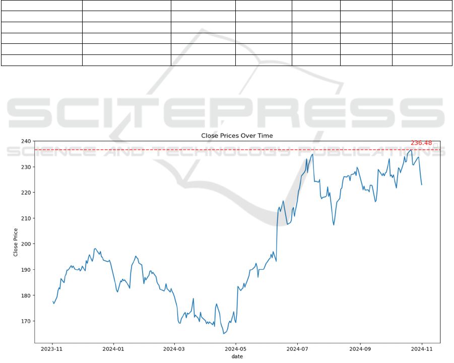
Figure 1: Close Prices Over Time. (Picture credit: Original)
Figure 1 shows the changes in stock closing prices
over a period. From November 2023 to November
2024, there were ups and downs in the stock prices.
The line on the graph shows the closing prices for
each day, and the red dotted line shows the highest
ICDSE 2025 - The International Conference on Data Science and Engineering
456

closing price, which is 236.48. According to Figure 1,
after reaching the lowest point in April 2024, the
stock prices started to go up and rose sharply after
May 2024. This might mean that during this time,
people's interest in this stock grew, leading to a higher
price.
Initial data processing and dataset division into
training and testing sets are part of the methodology.
Three regression models were employed: Random
Forest Regressor, Linear Regression, and XGBoost
Regressor, along with a combined model.
Classification models and voting classifiers were also
utilized to compare their performance. The combined
model was then used to predict the closing price five
days ahead.
2.2 Data Processing
2.2.1 Logarithmic Returns Calculation
To capture the percentage change in stock prices, this
paper calculate the logarithmic returns using
Equation (1).
𝐿𝑜𝑔𝑅𝑒𝑡𝑢𝑟𝑛

=ln
(
𝐶𝑙𝑜𝑠𝑒

)
−ln
(
𝐶𝑙𝑜𝑠𝑒

)(
1
)
This transformation helps stabilize the variance
and is commonly used in financial time series
analysis. The resulting series is denoted as log_return.
2.2.2 Augmented Dickey-Fuller Test
The log_return series is subjected to the Augmented
Dickey-Fuller (ADF) test to determine whether it is
stationary; the test statistic, p-value, and critical
values are extracted according to the test findings.
The time series is non-stationary, according to the
ADF test's null hypothesis; a series is considered
stationary if its p-value is less, often less than 0.05.
Table 2: The results of the ADF test.
ADF Statistic P value Critical values
-14.945638327 1.3028808059e-27
1% 5% 10%
-3.456780 -2.873171 -2.572968
The ADF test outcomes are displayed in Table 2,
which includes the ADF Statistic, P value, and
Critical values at different significance levels (1%,
5%, and 10%). The P value is incredibly small at
1.3028808059e-27, much below the conventional
threshold of 0.05, while the ADF Statistic is -
14.945638327. In contrast to the null hypothesis, this
suggests strong evidence that there are no stationary
time series. As a result, the series is deemed stagnant.
2.2.3 Moving Averages Calculation
To smooth the price data and capture trends, this
paper calculate the moving averages with different
window sizes by Equation (2).
M𝐴

=
1
𝑛
𝐶𝑙𝑜𝑠𝑒



(
2
)
In this formula, 𝑀𝐴

represents the moving
average on day n, n is the window size, and 𝐶𝑙𝑜𝑠𝑒

is
the closing price on day i. Specifically, this paper
compute: MA_5 (5-day moving average),MA_10
(10-day moving average),MA_30 (30-day moving
average) and MA_60 (60-day moving average).
2.2.4 Relative Strength Index Calculation
A momentum indicator called the Relative Strength
Index (RSI) gauges the size of the most current
pricing movements to identify whether the market is
overbought or oversold. It is created using equations
(3) and (4).
RSI=100 −
100
1+𝑅𝑆
(
3
)
where
RS=
𝐴𝑣𝑒𝑟𝑎𝑔𝑒𝐺𝑎𝑖𝑛
𝐴𝑣𝑒𝑟𝑎𝑔𝑣𝐿𝑜𝑠𝑠
(
4
)
Specifically, AverageGain is the average increase
in stock prices on days when the stock price went up
within a selected time period, and Average Loss is the
average decrease in stock prices on days when the
stock price went down within the same time period.
Higher RSI readings may indicate overbought
conditions, while lower values may indicate oversold
conditions. RSI values typically range from 0 to 100.
2.2.5 On-Balance Volume (OBV)
Calculation
OBV is a momentum indicator that relates price
changes to volume. It is calculated as shown in
Equation (5), Equation (6) and Equation(7) .
𝑂𝐵𝑉=𝑂𝐵𝑉

+𝑠𝑖𝑔𝑛
(
𝛥𝐶𝑙𝑜𝑠𝑒

)
×𝑉𝑜𝑙𝑢𝑚𝑒

(
5
)
where
Predicting Apple Inc. Stock Prices Using Machine Learning Techniques
457

Δ𝐶𝑙𝑜𝑠𝑒

=𝐶𝑙𝑜𝑠𝑒

−𝐶𝑙𝑜𝑠𝑒

(
6
)
𝑠𝑖𝑔𝑛
(
𝛥𝐶𝑙𝑜𝑠𝑒

)
=
1 𝛥𝐶𝑙𝑜𝑠𝑒

>0
−1 𝛥𝐶𝑙𝑜𝑠𝑒

<0
0 𝑜𝑡ℎ𝑒𝑟𝑤𝑖𝑠𝑒
(
7
)
𝑉𝑜𝑙𝑢𝑚𝑒

is the trading volume on day t.
2.2.6 Target Calculation
The target parameter is calculated as a binary label
indicating whether the following day's closing price
is higher than the current one. as Equation (8).
𝑇𝑎𝑟𝑔𝑒𝑡=
1 𝐶𝑙𝑜𝑠𝑒

>𝐶𝑙𝑜𝑠𝑒

0 𝑜𝑡ℎ𝑒𝑟𝑤𝑖𝑠𝑒
(
8
)
2.2.7 Feature Selecting
The selected features include 'Open', 'High', 'Low',
'Volume', 'Adj Close', moving averages (MA_5,
MA_10, MA_30, MA_60), Relative Strength Index
(RSI), and On-Balance Volume (OBV).
2.3 Machine learning methods
2.3.1 Random Forest Regressor
A method of group learning called the Random Forest
Regressor generates several different decision trees
throughout the training process and provides the
mean forecast for every tree. Equation (9) defines the
model.
𝑦=
1
𝑁
𝑇

(
𝑥
)


(
9
)
where 𝑇

(𝑥) is the i-th decision tree's forecast, and
N is the forest's tree count.
2.3.2 Linear Regression
Linear regression explains the relationship between a
dependent variable and one or more independent
variables by fitting a linear equation to observed data.
Equation (10) defines the model.
𝑦=𝑤

𝑥+𝑏
(
10
)
where b is the bias term, w is the weight vector,
and x is the feature vector.
2.3.3 XGBoost
XGBoost is a distributed gradient boosting toolkit
that has been improved for efficiency and scalability.
It uses a gradient boosting framework to build a
collection of inaccurate prediction models, usually
decision trees. The model is defined as Equation (11).
𝑦

=𝑦

+𝑓

(
𝑥

)


(
11
)
where 𝑓

represents the k-th decision tree and K is
the number of trees.
2.3.4 Combined Model
A combined model approach is used to integrate
predictions from the individual regression models.
The combined model is generated by giving different
weights to the prediction outcomes of each base
model and then computing the weighted average of
these forecasts. Specifically, the combined prediction
is calculated using Equation (12).
𝑦

=𝛼

(
𝑦

)


(
12
)
where 𝛼

are the weights given to each model
according to how well they perform.
The three base models selected for this paper are
the random forest regression model (Random Forest
Regressor), the linear regression model (Linear
Regression), and the Extreme Gradient Boosting
(XGBoost) regression model. These models were
chosen because of their excellent performance in
handling different types of data and problems. A
random forest ensemble learning technique generates
the class that is the average prediction (regression) or
the mode of the classes (classification) of each of the
decision trees. The independent and dependent
variables are assumed to have a linear relationship in
a simple prediction model known as linear regression.
A gradient boosting framework is used by the
effective machine learning method XGBoost to
maximize model performance.
To make predictions and determine each model's
performance metrics, such as Mean Squared Error
(MSE), Mean Absolute Error (MAE), and R-squared
(R^2), the program first trains each model using the
training dataset (X_train, y_train). It next utilizes the
testing dataset (X_test).
These metrics help evaluate each model's
predictive performance and determine the weights
that should be assigned to each model.
The program then computes the combined
model's prediction results and assesses the combined
model's performance using the same performance
metrics. The application then outputs the
ICDSE 2025 - The International Conference on Data Science and Engineering
458

performance metrics for each model and the
combined model for comparison.
2.3.5 Classification Models and Voting
Classifiers
To compare performance, classification models are
used alongside regression models. Voting classifiers
are employed to combine predictions from multiple
models, with two approaches considered: hard voting,
where the prediction is determined by the majority
vote of the classifiers, and soft voting, where the
prediction is based on the average of the predicted
probabilities.
3 RESULTS
For multi-step forecasting, the recursive prediction
method is used. The model predicts the subsequent
value, which is used to update the input
characteristics for the subsequent prediction phase,
beginning with the last known data point. For a
predetermined number of steps (5 days), this process
is repeated.
3.1 Results of the Regression Models
MSE, MAE, and R^2 were the three main metrics
used to assess the regression models' performance.
The predicted accuracy and goodness-of-fit of each
model are thoroughly evaluated by these criteria.
The combined model, which incorporates
predictions from the three separate models, obtained
a 𝑅

Score of 0.971396, an MAE of 0.624180, and an
MSE of 0.684853, as Table 3 illustrates. This
suggests that the combination strategy improves
overall forecast accuracy by utilizing the advantages
of several models.
Table 3: Regression Model Performance Metrics.
Model MSE MAE R2
Linear Re
g
ression 0.009831 0.092355 0.999589
Random Forest 0.819510 0.681290 0.965772
XGBoost 2.088564 1.089128 0.912768
Combined Model 0.684853 0.624180 0.971396
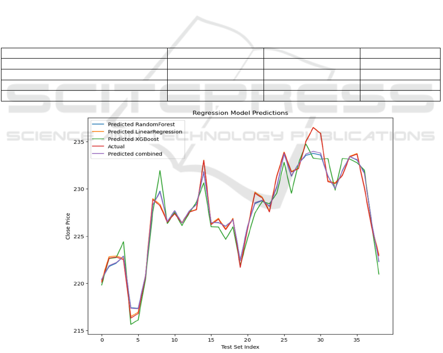
Figure 2: Regression Model Predictions. (Picture credit: Original)
A comparison between the actual values and the
expected results from different models is shown in
Figure 2. It is clear that the combined model (purple
line) closely tracks the actual values (purple line) in
most instances, indicating its high level of prediction
accuracy. Especially in regions where the data
Predicting Apple Inc. Stock Prices Using Machine Learning Techniques
459

experiences significant fluctuations, the prediction
curve of the combined model aligns well with the
actual values, showcasing its effectiveness in utilizing
the strengths of the other models and minimizing
potential biases from individual models.
3.2 Results of the Classifiers
3.2.1 Hard Voting Classifier vs. Soft Voting
Classifier
Table 4 and Table 5 show that both voting classifiers
have an accuracy of 0.5897, which means they
perform similarly when it comes to overall
classification accuracy. For both classes, the
precision and recall values of these two classifiers are
exactly the same: Class 1's precision is 0.69 and its
recall is 0.43, whereas Class 0's precision is 0.54 and
its recall is 0.78. Class 0 and Class 1 had F1-scores of
0.64 and 0.53, respectively. The F1-scores are
likewise identical.
This indicates that whether hard voting or soft
voting is used to combine the models, there is no
significant effect on the balance between precision
and recall for either class. All these experimental
results will be shown in a table to make them clearer.
Table 4: Hard voting classifier Performance.
Precision Recall F1-Score Support
Class 0 0.54 0.78 0.64 18
Class 1 0.69 0.43 0.53 21
accurac
y
0.59 39
macro avg 0.62 0.60 0.58 39
weighted avg 0.62 0.59 0.58 39
Table 5: Soft voting classifier Performance.
Precision Recall F1-Score Su
pp
ort
Class 0 0.54 0.78 0.64 18
Class 1 0.69 0.43 0.53 21
accurac
y
0.59 39
macro avg 0.62 0.60 0.58 39
wei
g
hted av
g
0.62 0.59 0.58 39
3.2.2 Voting Classifiers vs. Individual
Classifiers
Both voting classifiers (0.5897) have higher accuracy
compared to the individual classifiers (Random
Forest and XGBoost: 0.5641, Logistic Regression:
0.5385). This indicates that combining the predictions
of multiple models improves overall classification
performance.
Class 0 has a precision of 0.54 and recall of 0.78
in the voting classifiers, which is an improvement
over the individual models. The voting classifiers
show somewhat higher precision and recall for both
classes when compared to the individual classifiers.
The F1-scores for the voting classifiers are
slightly higher than those of the individual classifiers,
indicating a better balance between precision and
recall. Table 6 shows the classifier performance.
Table 6: Classifiers Performance.
Model
Precision (Class 0 / Class
1
)
Recall (Class 0 / Class
1
)
F1-Score (Class 0 /
Class 1
)
Accuracy
Random Forest 0.52 / 0.67 0.78 / 0.38 0.62 / 0.48 0.5641
Lo
g
istic Re
g
ression 0.00 / 0.54 0.00 / 1.00 0.00 / 0.70 0.5385
XGBoost 0.52 / 0.67 0.78 / 0.38 0.62 / 0.48 0.5641
Hard Voting
Classifie
r
0.54 / 0.69 0.78 / 0.43 0.64 / 0.53 0.5897
Soft Votin
g
Classifie
r
0.54 / 0.69 0.78 / 0.43 0.64 / 0.53 0.5897
ICDSE 2025 - The International Conference on Data Science and Engineering
460

4 CONCLUSIONS
Several machine learning models were used in this
study to predict future closing prices, and each
model's performance was assessed based on a wide
range of criteria. The results indicated that the
ensemble model approach, by integrating the
strengths of multiple individual models, provided
stable and consistent predictions for the next five
days. Specifically, the predicted closing prices for the
next five days were very close, demonstrating a stable
predictive trend. This stability is crucial for decision-
making in financial forecasting.
However, it must be recognized that although the
models demonstrated good performance, the real-
world financial markets are influenced by many
unpredictable factors. Therefore, while the ensemble
model offers valuable insights, its predictions should
be used in conjunction with other analytical tools and
expert judgment. Future work could include
incorporating more features, exploring different
model architectures, and conducting more extensive
backtesting to further enhance the model's predictive
accuracy and robustness.
REFERENCES
Chen, C.H. and Hsieh, C.Y. (2016). Actionable stock
portfolio mining by using genetic algorithms[J]. Inf.
Sci. Eng., 32(6), 1657–1678.
Chen, C.H. and Yu, C.H. (2017). A series-based group
stock portfolio optimization approach using the
grouping genetic algorithm with symbolic aggregate
approximations. Knowledge-Based Systems, 125, 146–
163.
Chou, Y.H., Kuo, S.Y., Chen, C.Y., and Chao, H.C. (2014).
A rule-based dynamic decision-making stock trading
system based on quantum-inspired tabu search
algorithm. IEEE Access, 2, 883–896.
Gunduz, H., Yaslan, Y., and Cataltepe, Z. (2017). Intraday
prediction of borsa istanbul using convolutional neural
networks and feature correlations. Knowledge-Based
Systems, 137, 138–148.
Hu, P., Pan, J.S., Chu, S.C., Chai, Q.W., Liu, T., and Li,
Z.C. (2019). New hybrid algorithms for prediction of
daily load of power network. Applied Sciences, 9(21),
4514.
Kim, K.j. and Han, I. (2000). Genetic algorithms approach
to feature discretization in artificial neural networks for
the prediction of stock price index. Expert systems with
Applications, 19(2), 125–132.
Long, W., Lu, Z., and Cui, L. (2019). Deep learning-based
feature engineering for stock price movement
prediction. Knowledge-Based Systems, 164, 163–173.
Rani, S. and Sikka, G. (2012). Recent techniques of
clustering of time series data: a survey. International
Journal of Computer Applications, 52(15).
Taylor, M.P. and Allen, H. (1992). The use of technical
analysis in the foreign exchange market. Journal of
international Money and Finance, 11(3), 304–314.
Wei Huang, Yoshiteru Nakamori, Shou-Yang Wang.
(2005). Forecasting stock market movement direction
with support vector machine, Computers & Operations
Research, 32, 2513-2522.
Predicting Apple Inc. Stock Prices Using Machine Learning Techniques
461