A Stock Price Trend Prediction Model Based on Tweet Sentiment

Analysis and Graph Convolutional Network

Yuning Zhu

School of Computer Science and Technology

, Tongji University, Jiading District, Shanghai, China

Keywords: Sentiment Analysis, Graph Convolutional Network, Knowledge Graph, Stock Price Movement Prediction.

Abstract: Public sentiment significantly affects investors’ decisions, often interfering with existing stock trends. In

recent years, indicators reflecting public sentiment have been introduced to assist in predicting stock

movements. Many studies have incorporated Graph Convolutional Network (GCN) to integrate this

influential factor for prediction, achieving highly competitive results. However, existing studies have

predominantly focused on official communication channels such as financial news, while neglecting in-depth

exploration of public attention dynamics and textual data from general netizens. This study analyzes

1,317,352 Twitter posts to extract their textual characteristics and sentiment attributes, evaluates influence

factors through interaction metrics, and constructs a knowledge graph integrated with stock market data.

Leveraging GCN's superior capability in modeling node relationships, this paper have effectively achieved

stock price trend prediction, demonstrating novel potential for knowledge graph applications in financial

forecasting. These findings suggest the potential benefits of incorporating diverse public sentiment sources

into stock prediction models and provide a foundation for further exploration of integrating social media

dynamics with financial forecasting.

1 INTRODUCTION

Predicting stock trends can help stakeholders make

informed investment decisions. Research indicates

that stock market prices are primarily influenced by

new information - such as news - rather than by

current or historical prices (Li et al., 2014). As news

events defy forecasting, stock markets exhibit random

walk dynamics - a phenomenon capping price

prediction accuracy at 50% statistically (Fama et al.,

1969).

An effective way to analyze this reflection of

public mood is to unscramble finance news collected

from social platform, i.e. twitter (Bollen, Mao, &

Zeng, 2011), into mood dimensions and adding these

labels to original stock data, which can significantly

improve the accuracy of the Dow Jones Industrial

Average (DJIA) predictions in Bollen et al.(2011)’s

research (Bollen, Mao, & Zeng, 2011). These

operations, known as sentiment analysis, have been

found to play a critical role in many applications such

as product reviews and restaurant reviews (Pang &

Lee, 2008; Liu & Zhang, 2012), and some researches

https://orcid.org/0009-0005-0613-5955

have tried to apply sentiment analysis on an

information source to improve the stock prediction

model (Nguyen, Shirai, & Velcin, 2015). Previous

works focused on opinion based sentiment analysis,

which integrates the textual information with the

historical prices through machine learning models or

deep learning models (Hu et al., 2018; Nguyen,

Shirai, & Velcin, 2015; Zhang et al., 2022), and

aspect based sentiment analysis, which assumes that

all words within a sentence comes from a single

subject (Nguyen, Shirai, & Velcin, 2015).

From a different angle, contemporary scholars

have tried to use stock relations to predict stock price

movements (SPMP). Graph convolutional networks

(GCN) (Kipf & Welling, 2016; Velickovic et al.,

2017), as potent structural data learners, excel at

modeling complex stock-factor relationships

underlying SPMP dynamics. For instance, Li et al.

addressed the impact of overnight financial news and

suggested an LSTM relational GCN model which

constructs relation specific graphs to aggregate node

semantics in text for SPMP (Li, Shen, & Zhu, 2018).

Cheng and Li suggested an attribute-driven graph

448

Zhu, Y.

A Stock Price Trend Prediction Model Based on Tweet Sentiment Analysis and Graph Convolutional Network.

DOI: 10.5220/0013699200004670

Paper published under CC license (CC BY-NC-ND 4.0)

In Proceedings of the 2nd International Conference on Data Science and Engineering (ICDSE 2025), pages 448-454

ISBN: 978-989-758-765-8

attention network to acquire relation embeddings via

attention mechanism and further aggregate attributes

by using GCN for SPMP in order to capture the

relation importance changing over time (Li et al.,

2020).Peng et al. investigated dual-type entity

relations -both implicitly and explicitly- and

developed a multi-attention neural framework that

incorporates internal and mutual impacts to

synthesize stock data for SPMP applications (Peng,

Dong, & Yang, 2023).

Compared to the above, the innovation points of

this paper include the following aspects: First, the

focus of this article is the collected tweet content of

the corresponding date in the stock time period and

the tweet interaction index. The processing method

proposed in this paper fully captures and takes into

account each feature of the tweet data, including

using the Bidirectional Encoder Representation from

Transformer(BERT) model to expand the tweet text

feature, using sentiment analysis method combined

with multiple interaction indexes to score the tweet

emotion and influence weights. Secondly, unlike

previous work, this paper will keep the tweets and

stock characteristics independently, establishing the

relationships between the two through the

construction of knowledge graph, and capture its

internal correlation characteristics using the GCN

network. This paper innovatively establishes a

pathway from raw tweet data to knowledge graph

construction, ultimately leading to stock price trend

prediction results.

2 DATA AND METHOD

2.1 Data Collection and Description

This research first uses the Twitter Financial News

Sentiment Dataset(dataset 1, shown in table 1) and the

Natural Language Toolkit (NLTK) package to train

and predict the mood of news collected in the Tweets

about the Top Companies from 2015 to 2020

dataset(dataset 2, shown in table 2) as sentiment

features, combined with the APPLE Stock

Data(dataset 3, shown in table 3) to predict future

trends. Labels in table 1 are explained in table 5.

Table 1: Twitter Financial News Sentiment Dataset.

text label

$BYND - JPMor

an... 0

“The worst is behind us... 1

Time: 15:00 #Stoc

... 2

Tables 1, 2 and 3 respectively demonstrated the

datasets used for sentiment analysis, tweet selection,

and stock data processing. These three datasets will

be used in sequence during the subsequent

experimental processes.

2.2 Method

Table 2: Tweets about the Top Companies from 2015 to 2020.

tweet i

write

ost date

comment retweet like

550441509175443456 VisualStockRSRC 1420070457

lx21 made $10,008 on

$AAPL...

0 0 1

550441672312512512 KeralaGuy77 1420070496

Insanity of today

weirdo massive selling...

0 0 0

Table 3: APPLE Stock Data

Date O

en Hi

h Low Close Ad

Close Volume

1980-12-12 0.128348 0.128906 0.128348 0.128348 0.100323 469033600

1980-12-15 0.12221 0.12221 0.121652 0.121652 0.095089 175884800

1980-12-16 0.113281 0.113281 0.112723 0.112723 0.08811 105728000

1980-12-17 0.115513 0.116071 0.115513 0.115513 0.090291 86441600

1980-12-18 0.118862 0.11942 0.118862 0.118862 0.092908 73449600

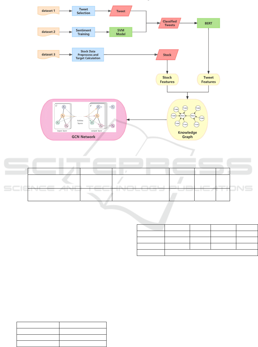
This paper innovatively proposes a processing

workflow for predicting stock trends using tweet data

and sentiment analysis, as shown in Figure 1. First,

the dataset is preprocessed by selecting tweets,

training sentiment classifier and processing technical

indicators and target for stock data. Next, a

heterogeneous graph knowledge graph is constructed.

Finally, the knowledge graph is used as input to enter

a heterogeneous graph convolutional neural network

for training and prediction.

2.2.1 Selection of Tweets

Tweets are related to a company in dataset 2 through

tweet id. In this section, tweets’ date are first

formatted into datetime, then tweets about Apple

A Stock Price Trend Prediction Model Based on Tweet Sentiment Analysis and Graph Convolutional Network

449

Inc.(ticker symbol: AAPL) are selected uniquely.

1,317,352 distinct tweets from 2015-01-01 to 2020-

01-01 of AAPL are selected as final tweets, with an

example shown in table 4.

Figure 1: Overall Process. (Picture credit: Original)

Table 4: Tweets about AAPL.

tweet id post date body comment retweet like

550441509175443456 1420070457

lx21 made $10,008 on

$AAPL...

0 0 1

550441672312512512 1420070496

Insanity of today

weirdo massive selling...

0 0 0

2.2.2 Sentiment Training

In sentiment training section, a support vector

machine(SVM) is trained to categorize tweets into

sentiment labels using dataset 1 and NLTK package.

The model achieved an overall accuracy of

82.96%, with a detailed classification report in table

6. Using the trained SVM model, tweets(shown in

table 4) are classified into one of the three labels in

table 5 (with each label representing the attitude of the

tweet towards a certain stock), combined with its

original date, body, comment number, retweet

number and like number (examples are shown in table

7). These processed tweet data will be preserved for

the construction of knowledge graph.

Table 5: Sentiment Labels.

label sentiment

0 Bearish

1 Bullish

2 Neutral

Table 6: Classification report of Sentiment Training.

class

recision recall F1-score support

Bearish 0.7233 0.5274 0.6100 347

Bullish 0.7937 0.6884 0.7373 475

Neutral 0.8537 0.9393 0.8945 1566

Accurac

82.96%

As can be seen from Table 6, the overall accuracy

rate of the model for sentiment classification is

82.96%. Among them, the model's recognition effect

for Neutral sentiment is the best, with relatively high

precision, recall and F1 score. This could possibly be

because there are more samples of this category in the

data, and thus the model's predictions are more biased

towards this category. In contrast, the recognition

effect for the Bearish category is poorer. Although its

precision reaches a moderate level, the recall rate

remains relatively low, and the F1-Score

is moderately low, indicating that the model has a

certain degree of misjudgment in identifying Bearish

ICDSE 2025 - The International Conference on Data Science and Engineering

450

samples and is prone to missing some actual Bearish

sentiments. However, on the whole, the model's high

recognition effect has not been significantly affected

by class imbalance, meaning that the model has strong

robustness and stability in this sentiment

classification task.

2.2.3 Stock Preprocessing and Target

Calculation

In this section, log returns are first calculated using

formula 1, where Pt is the present Adjusted Close

(Adj Close) price, and Pt-1 is the Adj Close price of

its previous date:

Log Return = ln





= ln

(



)

− ln

(



)

(1)

Statistics of the Augmented Dickey Fuller Test

(ADF Test) are shown in table 8. The results indicate

a rejection of the null hypothesis of non-stationarity,

which suggests that the time series is likely stationary.

Table 7 show the processed tweets about AAPL.

Table 7: Processed Tweets about AAPL.

ost date

ody

redicted label comment retweet like

2015-01-01 lx21 made $10,008 on $AAPL... 2 0 0 1

2015-01-01 Insanit

of toda

weirdo massive sellin

... 1 0 0 0

2015-01-01 Swing Trading: Up To 8.91% Return In... 2 0 0 1

Table 8: ADF Test Results.

metric ADF Statistic p-values critical values (1%) critical values (5%) critical values

(10%)

value -10.5651 7.5529e

-19

-3.4356 -2.8639 -2.5680

Finally, the target for prediction -the movement

direction (up or down) of the stock in the next day,

where the stock data of open, high, low, close and

volume are unknown- is calculated with formula 2,

where t stands for current day, 0 stands for down, and

1 stands for up. Additionally, in order to achieve a

balanced distribution of target, a threshold of 0.8% is

set to identify the direction of stock (Li et al., 2014;

Fama et al., 1969).

target = 

0 if ln

Adj Close





Adj Close



≤threshold

1 otherwise

(2)

Target calculation resulted in a balanced distri-

bution of 50.35% ups and 49.65% downs.

2.2.4 Construction of Knowledge Graph

The proposed model is as follows: First, 1,257 stock

data and 1,317,352 tweets are initialized as nodes of

the knowledge graph in time series. Stock class nodes

have seven dimensions, namely open, close, adj close,

high, low, volume and log return. Tweet class nodes

have features of 768 dimensions obtained by the NLP

model BERT by processing the original body text of

the tweets. The corresponding features and feature

dimensions of different types of nodes are displayed

in table 9.

Table 9: Features and Dimensions.

node t

e features dimensions

stock

open, close, adj close,

high, low, volume, log

return

tweet obtained by BERT 768

Next, the edge relationship between these nodes is

established. Two types of edges are designed.

The first type of edges is the Tweet-influences-

stock edge, where tweets posted in one day are

connected to the stock node of its post date, each

tweet-influences-stock type edge weight reflects the

public attention through comprehensive considera-

tion of sentiment classification and interactive

number (including like, comment and retweet

number), which eventually formed 1,079,871 rela-

tionship edge and corresponding weight. Weights are

calculated using formulas 3 and 4.

Among them, attention N(c,r,l) is obtained by the

weighted sum of comments, the number of retweets

and the number of likes. Furthermore, W(s,c,r,l)

represents the edge weight of tweet-influences-stock,

𝛿



is the negative sentiment weight, 𝛿



is the positive

sentiment weight, δ is the neutral sentiment weight,

and attention N(c,r,l) is calculated by formula 3. For

tweets with neutral emotions, it is considered that the

higher the attention, the closer the emotion is to

positive.

A Stock Price Trend Prediction Model Based on Tweet Sentiment Analysis and Graph Convolutional Network

451

The second type of edges is the Stock-related-

stock edge. The establishment of a tweet-influences-

stock relationship considers the impact of public

sentiment on the day, while stock-related-stock

relations consider the impact of past historical data on

the future. For each stock node, stock nodes within a

specific history window (after experiments, the

history window selected in this article is 5 days) is

connected to the node (setting self-loops for its own

node), and the closer the historical node is to the

present node, the greater the impact, and the weight

increases accordingly.

2.2.5 Feature Extension by BERT

The characteristics of the original tweet (which has

been retained through the tweet node relationship

when the knowledge graph is established) are: body,

predicted_label, comment_num, retweet_num, like_

num. The last four features have been fully considered

when calculating the knowledge graph weight, while

‘body’, namely the original content of the tweet, has

not been considered. Using BERT, the content of

tweet are disposed through the text vectoring,

resulting in 768 dimensions of tweet features. These

features, after normalization, serve as input for the

subsequent tweet section of the graph convolution

network.

2.2.6 Graph Convolutional Network

The network used in this article is composed by

different heterogeneous graph convolutional neural

models.

First, the graph data will be entered to the GAT

layer. The GAT model used in this layer introduces a

mechanism of multi-head attention, updating the

tweet-influences-stock relationship of the input

through two attention heads. This layer will transfer.

(

c,r,l

)

= α∙c+β∙r+γ∙l

(

)

(

s,c,r,l

)

= 



∙ N

(

c,r,l

)

predicted





earish





∙ N

(

c,r,l

)

predicted





ullish



δ∙N

(

c,r,l

)

+ε∙1+N

(

c,r,l

)

 predicted





eutral



(

)

the characteristics of each tweet node to the stock

node through the edges, and splicing the output of the

two attention heads in a means aggregation way. The

function of this layer is to pass the unrelated tweet

features in the same day to the stock node, and output

the updated stock features. Considering that the

feature dimension of tweet nodes is large, and the

adjacency matrices of the stock nodes are relatively

sparse, this paper conducted experiments on both

GAT model and SAGE model on the model selection

of this layer. The results show that the training result

model obtained using GAT model can converge,

while the model cannot converge using SAGE model.

The reason for this result may be that SAGE reduces

the complexity of the model by sampling nodes.

However, since the characteristics of tweet nodes are

one of the important dimensions of the model, the

whole graph cannot be transmitted through SAGE

network alone, resulting in poor effect.

The output of the previous layer will only contain

the updated stock node features. The output was then

activated and dropped out.

The second convolutional layer is the SAGE layer.

In the input of this layer, for each stock node, its

characteristics have included the tweet features

updated by the first convolutional layer, as well as the

stock-related-stock relationship and weights

constructed above. The reason why SAGE is selected

in this layer is that the SAGE model only transmits

messages to its K-order neighbors. When establishing

the heterogeneous knowledge graph, in order to avoid

interference between stock nodes with a long time

interval, each stock node is only associated with its 5

historical nodes to retain the influence of a specific

time window. The SAGE model selected by this layer

also only updates the first order neighbor information

of each stock node, combined with heterogeneous

knowledge graph, that is, only 5 historical nodes are

transmitted.

The output is activated next. After activation, the

BatchNorm layer is used to normalize the data. The

classification results are finally outputed using

softmax.

3 RESULTS AND DISCUSSION

3.1 Experimental configuration

The training set used in the experiment was 90% of

the original data set, and the test set was 10% of the

original data set. The experimental configurations are

shown in the table 10.

ICDSE 2025 - The International Conference on Data Science and Engineering

452

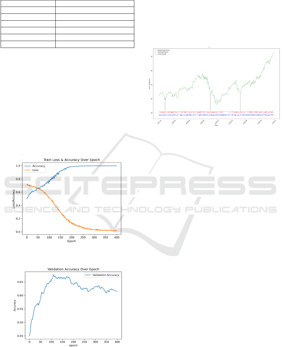
Table 10: Experimental Configurations

metric confi

uration

timize

Adam

Learnin

rate 0.0003

Loss Negative Log Likelihood Loss

Epoch 400

Early stop 200

Dro

Out 0.5

3.2 Results

The accuracy and loss of the training set during the

experiment is shown in figure 2, and the accuracy of

the validation(test) set is shown in the figure 3. After

experiments, the accuracy of this model can reach up

to 67.46% on the test set, and the accuracy of the

training set is 79.49% at the same time. As the training

epoch increased, the model subsequently showed an

overfitting trend despite the use of overfi-

tting prevention measures such as dropout and early

stop. The training set gradually converged to the acc-

uracy of 100%, but the performance of the test set

gradually decreased.

Figure 2: Train Loss and Accuracy Oveer Epoch (Picture

credit: Original)

Figure 3: Validation Accuracy Over Epoch (Picture credit:

Original)

Real stock prices(green), true stock trends(blue),

and forecast stock trends(red) from 2017 to 2019 are

shown in figure 4. Presented in the figure, the

predicted trend and real trend are almost consistent,

especially when sharp turnings occurred, which are

highlighted by the dashed line. However, the

performance of the model still fluctuates and overfits,

and there is room for improvement.

Figure 4: Real stock prices, True stock trends and Forecast

stock trends (Picture credit: Original)

4 CONCLUSIONS

In conclusion, the method proposed in this article can

effectively predict the stock price trend through

public sentiment indicators and data input when

future data is unknown. In the occurrence of

important news events and major transitions of stock

prices, the model combined with the public senti-

ment analysis can effectively predict the turning

point. Compared to approaches that solely rely on

sentiment classification of tweet texts, this paper

integrates both sentiment and influence analysis of

tweets and incorporates knowledge graphs into GCN

networks, which enhances the model’s predictive

performance. By synergizing these dual consid-

erations, this approach offers novel possibilities for

leveraging knowledge graphs in the field of stock

trend prediction. However, the current model relies

on extensive textual input and computationally

intensive BERT-based processing, while its general-

izability remains limited. Future applications of this

model could focus on predicting stock trends during

major news events. Future work will include

improving the universality of the model, as well as

further exploring the application of GCN and deep

learning models in this prediction mode.

A Stock Price Trend Prediction Model Based on Tweet Sentiment Analysis and Graph Convolutional Network

453

REFERENCES

Bollen, J., Mao, H., & Zeng, X. (2011). Twitter mood

predicts the stock market. Journal of Computational

Science, 2(1), 1-8.

Fama, E. F., Fisher, L., Jensen, M. C., & Roll, R. (1969).

The adjustment of stock prices to new information.

International Economic Review, 10(1), 1-21.

Hu, Z., Liu, W., Bian, J., Liu, X., & Liu, T. Y. (2018,

February). Listening to chaotic whispers: A deep

learning framework for news-oriented stock trend

prediction. In Proceedings of the Eleventh ACM

International Conference on Web Search and Data

Mining (pp. 261-269).

Li, H., Shen, Y., & Zhu, Y. (2018, November). Stock price

prediction using attention-based multi-input LSTM. In

Asian Conference on Machine Learning (pp. 454-469).

PMLR.

Li, Q., Tan, J., Wang, J., & Chen, H. (2020). A multimodal

event-driven LSTM model for stock prediction using

online news. IEEE Transactions on Knowledge and

Data Engineering, 33(10), 3323-3337.

Li, Q., Wang, T., Li, P., Liu, L., Gong, Q., & Chen, Y.

(2014). The effect of news and public mood on stock

movements. Information Sciences, 278, 826-840.

Liu, B., & Zhang, L. (2012). A survey of opinion mining

and sentiment analysis. Mining Text Data, 415-463.

Nguyen, T. H., Shirai, K., & Velcin, J. (2015). Sentiment

analysis on social media for stock movement prediction.

Expert Systems with Applications, 42(24), 9603-9611.

Pang, B., & Lee, L. (2008). Opinion mining and sentiment

analysis. Foundations and Trends® in Information

Retrieval, 2(1–2), 1-135.

Peng, H., Dong, K., & Yang, J. (2023). Stock price

movement prediction based on relation type guided

graph convolutional network. Engineering Applications

of Artificial Intelligence, 126, 106948.

Zhang, Q., Qin, C., Zhang, Y., Bao, F., Zhang, C., & Liu,

P. (2022). Transformer-based attention network for

stock movement prediction. Expert Systems with

Applications, 202, 117239.

Veličković, P., Cucurull, G., Casanova, A., Romero, A.,

Lio, P., & Bengio, Y. (2017). Graph attention networks.

arXiv preprint arXiv:1710.10903.

Kipf, T. N., & Welling, M. (2016). Semi-supervised

classification with graph convolutional networks. arXiv

preprint arXiv:1609.02907.

ICDSE 2025 - The International Conference on Data Science and Engineering

454