Space-Filling Regularization for Robust and Interpretable

Nonlinear State Space Models

Hermann Klein

, Max Heinz Herkersdorf

and Oliver Nelles

University of Siegen, Department Mechanical Engineering, Automatic Control – Mechatronics,

Paul-Bonatz-Str. 9-11, 57068 Siegen, Germany

Keywords:

Nonlinear System Identiﬁcation, State Space Models, Regularization, Local Model State Space Network,

Space-Filling.

Abstract:

The state space dynamics representation is the most general approach for nonlinear systems and often chosen

for system identiﬁcation. During training, the state trajectory can deform signiﬁcantly leading to poor data

coverage of the state space. This can cause signiﬁcant issues for space-oriented training algorithms which

e.g. rely on grid structures, tree partitioning, or similar. Besides hindering training, signiﬁcant state trajectory

deformations also deteriorate interpretability and robustness properties. This paper proposes a new type of

space-ﬁlling regularization that ensures a favorable data distribution in state space via introducing a data-

distribution-based penalty. This method is demonstrated in local model network architectures where good

interpretability is a major concern. The proposed approach integrates ideas from modeling and design of

experiments for state space structures. This is why we present two regularization techniques for the data point

distributions of the state trajectories for local afﬁne state space models. Beyond that, we demonstrate the

results on a widely known system identiﬁcation benchmark.

1 INTRODUCTION

Models of dynamic systems are the base for numerous

industrial applications, especially for control design

or virtual sensing. Insofar as white box models de-

rived from physical principles oftentimes fail to meet

an acceptable tradeoff between modeling effort and

accuracy, data-driven model learning, also known as

system identiﬁcation, comes into play. Here, the user

can choose between different mathematical architec-

tures to describe the system’s dynamics. A state space

representation is the most abstract and general kind

as well as required for many control design methods.

Examples of alternative approaches are feedforward-

trained models like ﬁnite impulse response or non-

linear autoregressive models with exogenous input or

output feedback-trained kinds like output error mod-

els (Ljung, 1999). In comparison to the latter and es-

pecially for the nonlinear case, the state space model

is a more powerful modeling approach due to its inter-

nal state feedback (Belz et al., 2017; Sch

ussler et al.,

2019).

https://orcid.org/0009-0009-5386-3575

https://orcid.org/0009-0007-8554-8153

https://orcid.org/0000-0002-9471-8106

Whereas linear state space models can be ex-

tracted from frequency domain approaches with sub-

space identiﬁcation (Pintelon and Schoukens, 2012;

Van Overschee and De Moor, 1995), nonlinear mod-

els have to be trained via nonlinear optimization with

the objective of simulation error ﬁt. They gener-

ally arise when the linear state and output functions

are replaced with nonlinear function approximators.

Here, various approaches exist, including polynomi-

als (Paduart et al., 2010) or neural networks (Suykens

et al., 1995; Forgione and Piga, 2021). Due to local

interpretability and explainability reasons, we focus

on the class of local afﬁne state space models. Math-

ematically related architectures are (softly switching)

piecewise afﬁne (Garulli et al., 2012), Takagi Sugeno

(TS) or quasi-Linear Parameter Varying (qLPV) state

space models (Rotondo et al., 2015).

In general, system identiﬁcation tries to ﬁnd

an accurate model based on input/output training

datasets (Ljung et al., 2020). As a consequence, an

immanent feature of nonlinear state space models is

the implicit optimization of the model’s state, since it

depends on trainable parameters. Due to the simula-

tion error ﬁt, the state is optimized indirectly. In ge-

ometrical terms, deformations of the trajectories can

Klein, H., Herkersdorf, M. H. and Nelles, O.

Space-Filling Regularization for Robust and Interpretable Nonlinear State Space Models.

DOI: 10.5220/0013698800003982

Paper published under CC license (CC BY-NC-ND 4.0)

In Proceedings of the 22nd International Conference on Informatics in Control, Automation and Robotics (ICINCO 2025) - Volume 1, pages 409-416

ISBN: 978-989-758-770-2; ISSN: 2184-2809

409

be observed within the optimization procedure. This

can be visualized in the phase plot of the state vari-

ables’ trajectories, at least for the two-dimensional

projection

. The point distribution in the state space is

manipulated until the termination of the optimization.

For TS models, the effects on the state trajectory can

be connected with local regions. This interaction can

affect robustness and interpretability and is addressed

in this contribution.

As a ﬁrst try, any system identiﬁcation task can

be challenged with a pure data-driven (black box) ap-

proach. In such a setting, the state space model is

fully parametrized including redundant parameters. A

common technique in estimation theory is to use regu-

larization by application of an additional penalty term

to the objective function (Boyd and Vandenberghe,

2004). In the context of nonlinear state space mod-

eling, recent work deals with L1 regularization for

black box models (Bemporad, 2024). Moreover, Liu

et al. (2024) use regularization to make a black-box

state meet a physical-interpretable state realization.

An overview on methods for nonlinear systems can

e.g. be found in Pillonetto et al. (2022).

As mentioned above, the interaction of the data

point distribution with local activation functions is

crucial for models with regional organization, like the

Local Model State Space Network (LMSSN). As a

consequence, we develop a space-ﬁlling regulariza-

tion for the LMSSN procedure. This transfers ideas

from the Design of Experiments into model training.

The novelty of this contribution is the development of

a space-ﬁlling penalty term. We analyze it in detail

and compare two related regularization techniques.

The article is organized as follows. In Section 2,

we present the LMSSN-based modeling procedure.

Next, we present the evolution of the space-ﬁlling

indicators within the optimization procedure in Sec-

tion 3. The effect of a space-ﬁlling penalty term is

presented in Section 4. Our method is tested on a

benchmark process in Section 5. Finally, we summa-

rize our work and give an outlook on future lines of

research.

2 NONLINEAR STATE SPACE

MODELING

The proposed method is suitable for all state space

models in which the state explores an a priori known

range. Since we focus on the LMSSN method, its

functionality is introduced in this section. This un-

For simplicity, the phase plot of the state variables is

designated as the state trajectory in this paper.

regularized version serves as a reference for recent

advancements regarding space-ﬁlling regularization.

2.1 Local Model State Space Network

LMSSN is a system identiﬁcation method to create

discrete-time nonlinear state space models. The math-

ematical model architecture embeds Local Model

Networks (LMNs) in a state space framework.

LMSSN modeling results in local afﬁne state space

models, weighted with normalized radial basis func-

tions (NRBF). Detailed information can be found

in Sch

ussler (2022). It is emphasized that LMSSN

differs from TS and qLPV approaches in the use of

the Local Linear Model Tree (LOLIMOT). The tree-

construction algorithm serves for the determination

of the fuzzy premise variables (or scheduling vari-

ables in qLPV terms). Additionally, it uses a heuris-

tic axis-orthogonal input space partitioning approach

by automatic parametrization of the validity func-

tions. For more information about LOLIMOT, we re-

fer to Nelles (2020).

The resulting LMSSN model is formulated with

the following equations,

ˆx(k + 1) =

LM,x

∑

j=1

ˆx(k) + b

u(k) + o

) ◦ Φ

[x]

(k)

ˆy(k) =

LM,y

∑

j=1

⊤

ˆx(k) + d

u(k) + p

) ◦ Φ

[y]

(k).

(1)

For the single-input single-output case (n

=1 input

and n

=1 output variable), the tensors A

∈ R

×n

∈ R

, o

∈ R

, c

∈ R

, d

∈ R and p

∈ R

are ﬁlled with the slopes and offsets of the j-th lo-

cal afﬁne model (LM). The dynamical order is ex-

pressed by the number of state variables n

and the

discrete-time is indicated with k. In conﬁguration (1),

there are altogether n

LM,x

superposed afﬁne models

for the state ˆx(k + 1) and n

LM,y

for the output ˆy(k).

The basis functions Φ

[x]

and Φ

[y]

express the j-th local

validity function. Since they are implemented with

normalized Gaussians, the partition of unity holds,

∑

LM,x

j=1

[x]

= 1 and

∑

LM,y

j=1

[y]

= 1.

Due to the design of LMSSN in state space form,

the parameter initialization can be done determinis-

tically with a global linear state space model. The

latter is gathered as the Best Linear Approximation

(BLA) of the process in the frequency domain (McK-

elvey et al., 1996). Next, subspace-based identiﬁca-

tion converts the nonparametric frequency response

function model into a parametric linear state space

model. The fully-parametrized discrete-time model is

then transformed into a balanced realization via a sim-

ICINCO 2025 - 22nd International Conference on Informatics in Control, Automation and Robotics

410

ilarity transformation (Verriest and Kailath, 1983; Lu-

enberger, 1967). It evokes a diagonal structure within

the state space matrices which leads to a state real-

ization with an evenly (and thus desired) trajectory

shape.

After the linear model initialization, the

LOLIMOT algorithm starts. With the help of

the stepwise addition of weighted LMs, it enables

for nonlinear curve approximation. Each LM is

connected with a region of activation in the extended

input/state space ˜u = [ ˆx,u]

. This corresponds to the

partition of ˜u with interpolation regimes for smooth

cross-fading in between. It can be seen as a genera-

tion of splits of ˜u, arranged by center placement of the

NRBFs. If every dimension of ˜u is to be analyzed in

form of a split, n

Split

=dim(˜u) split options arise. For

the ease of the center placement, it is intuitive to scale

the state trajectory into a ﬁxed interval, preferably

the unit cube. The scaling is actualized with an afﬁne

scaling transformation, parametrized with range and

offset values according to minimum and maximum of

ˆx. The procedure is called split-adaption algorithm

according to Sch

ussler et al. (2019). Each LOLIMOT

iteration investigates all n

Split

options for the region

with the largest error separately via an optimization

run.

2.2 Problem Statement

The loss function J being minimized in each

LOLIMOT iteration is the sum of the squared output

errors. For a one-dimensional output variable, the op-

timization problem is stated as

min

J(θ ) = min

∑

k=1



y(k) − ˆy(k; θ )



s.t. ˆx(k + 1) = LMN(ˆx(k), u(k); θ

[x]

)

ˆy(k) = LMN( ˆx(k), u(k); θ

[y]

(2)

where θ is the vector of all model parameters and N

is the number of samples collected for training. The

nonlinear problem is solved with a Quasi-Newton op-

timizer with BFGS Hessian approximation. The op-

timization is run till convergence in a local minimum

terminating on a loss and gradient tolerance or mini-

mal step size.

By ﬁtting the parameters according to the min-

imization of the output error, the state trajectory

changes its shape from the balanced realization to

the one that is most effective for the objective (2).

Next, we show a possible consequence on the state

Note the LOLIMOT iterations have to be distinguished

from the gradient-based iterations within the nonlinear op-

timization of each split option.

trajectory for the ﬁrst split of a simulated second-

order single-input single-output system with nonlin-

ear feedback,

¨y(t) + a

˙y(t) + a

f (y(t)) = b

u(t), (3)

with the parameter values a

=15 and a

=3. The

nonlinear feedback f (y) is arranged with a smooth ex-

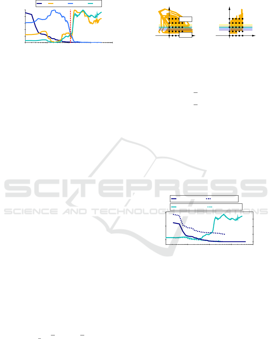
ponentially rising curve. Figure 1 demonstrates that

the initial state trajectory was within the unit cube,

whereas the optimized one is compressed. Obviously,

the nonlinear behavior of the process can be captured

although no data point is fully active in the upper

LM. Nevertheless, LM2 inﬂuences the data points via

smooth cross-fading of both LMs in the interpolation

regime. The shown behavior causes problems regard-

ing interpretation. Furthermore, the effect is accom-

panied by robustness problems. Large local parameter

values of LM2 are necessary to inﬂuence data, which

are located in the lower LM1. With the help of the

maximum absolute value of the eigenvalues µ

of the

local state transition matrices,

LM, j



⊤

1, j

⊤

2, j



unstable poles in LM2 can be detected:

max



LM,1

)



= 0.99 < 1,

max



LM,2

)



= 4.23 > 1

The phenomenon can be seen as overﬁtting and con-

tains the risk of unstable extrapolation behavior. Fi-

nally, the risk of reactivation (Nelles, 2020) of LMs

within the next splits is increased, since the split adap-

tion leads to major differences in the NRBF’s standard

deviations.

Figure 1: Extended state trajectory before ( ) and after ( )

the optimization of the ﬁrst split in the ˆx

-dimension. The

colored contour lines show the validity functions and mark

the interpolation regime. For brevity, the ˆx

-u projection is

left out.

Note that the ﬁxed centers of the LOLIMOT-

partitioned state space make this effect visible. It

can hardly be investigated for deep neural state space

models or recurrent neural networks, where all neu-

ral weights are trainable parameters. Furthermore, it

Space-Filling Regularization for Robust and Interpretable Nonlinear State Space Models

411

must be mentioned that the observed behavior (Fig. 1)

enables modeling with low ﬂexibility. In the case of

LMSSN this means that only one split is sufﬁcient for

the complete identiﬁcation. Thus it is very effective

because only two local linear models are able to ﬁt a

process with a smooth curve (3).

3 SPACE-FILLING EVOLUTION

Before merging modeling with space-ﬁlling proper-

ties, three suitable metrics for the assessment of data

point distributions are presented. Afterwards, their

evolution along the optimization progress is demon-

strated. For mathematical reasons, the state trajectory

is described as the set of points in the extended in-

put/state space as

X = ˜u

(k), ∀k ∈ {1, .. ., N}.

3.1 Metrics and Indicators

Inspired by the shape of the state trajectory in Fig. 1,

the covered volume is an intuitive and straightfor-

ward space-ﬁlling indicator. It can be assessed as

the volume of a convex hull on the state trajectory

(CHV) (Boyd and Vandenberghe, 2004). Written for

the extended input/state space, the volume V is de-

ﬁned as

V =

dim( ˜u)

det(G),

(4)

where the Gram matrix G is ﬁlled with

i, j

= ˜u(i)

˜u( j), ∀i, j ∈ H .

The convex hull is deﬁned by the set of points H ⊆

{1,2,...,N} derived with the help of the quickhull

algorithm. Intuitively, the CHV is going to deliver

large values for widely distributed points and small

values for concentrated points.

Alternatively, support point-based indicators are

commonly applied for assessing space-ﬁlling mea-

surements. Here, the state trajectory is compared to

a given distribution of n

grid or Sobol points G . In

this contribution, we concentrate on a uniform grid,

implying that a uniform distribution is desired. This

leads to the ﬁnal two metrics.

First, the mean of the minimum distances ψ

from

every grid point g

,∀ j ∈ { j = 1,2, .. ., n

}, to the

nearest extended input/state space point ˜u(k) is cal-

culated (Herkersdorf and Nelles, 2025). The criterion

is strongly related to Monte Carlo Uniform Sampling

Distribution Approximation (Smits and Nelles, 2024).

In this paper, it is denoted with ψ

and given as

∑

j=1

min

k∈{1,...,N}

d( ˜u(k),g

) (5)

with the Euclidian distance d

d( ˜u(k),g

) =

˜u(k) − g

)

( ˜u(k) − g

It is imporant to note that distance-based criteria such

as ψ

can encounter difﬁculties in high-dimensional

spaces. Furthermore, its grid-oriented nature is af-

fected by the curse of dimensionality. Both aspects

are beyond the scope of this work, as we focus on

lower-dimensional problems. Nonetheless, they con-

stitute limitations of the approach.

Secondly, from a statistical point of view, the

Kullback-Leibler Divergence (KLD) is able to as-

sess the similarity of two probability density func-

tions (PDF) Kullback and Leibler (1951) The PDF

of a dataset S is denoted by P(S ). In the preva-

lent application, it compares the estimated probabil-

ity density

P(X ) with the uniform distribution of a

grid P(G ) = 1/n

. The KLD is then calculated as

KLD = −

∑

k=1

log



P(X )



. (6)

The required probability density estimation of the

state trajectory is done with kernel density estima-

tion (Scott, 1992). For the measurement of the space-

ﬁlling properties of a point distribution, both KLD

and ψ

will decrease when the state trajectory be-

comes uniformly, i.e., meets the grid.

3.2 Tracking Within Nonlinear

Optimization

For the sake of plausibility, the previously introduced

indicators in the example depicted in Fig. 1 are ex-

amined. Obviously, CHV decreases as the optimiza-

tion progresses. On the other hand, KLD and ψ

are expected to grow, because the state trajectory

is evenly distributed before the optimization, and

narrow-shaped after the optimization has converged.

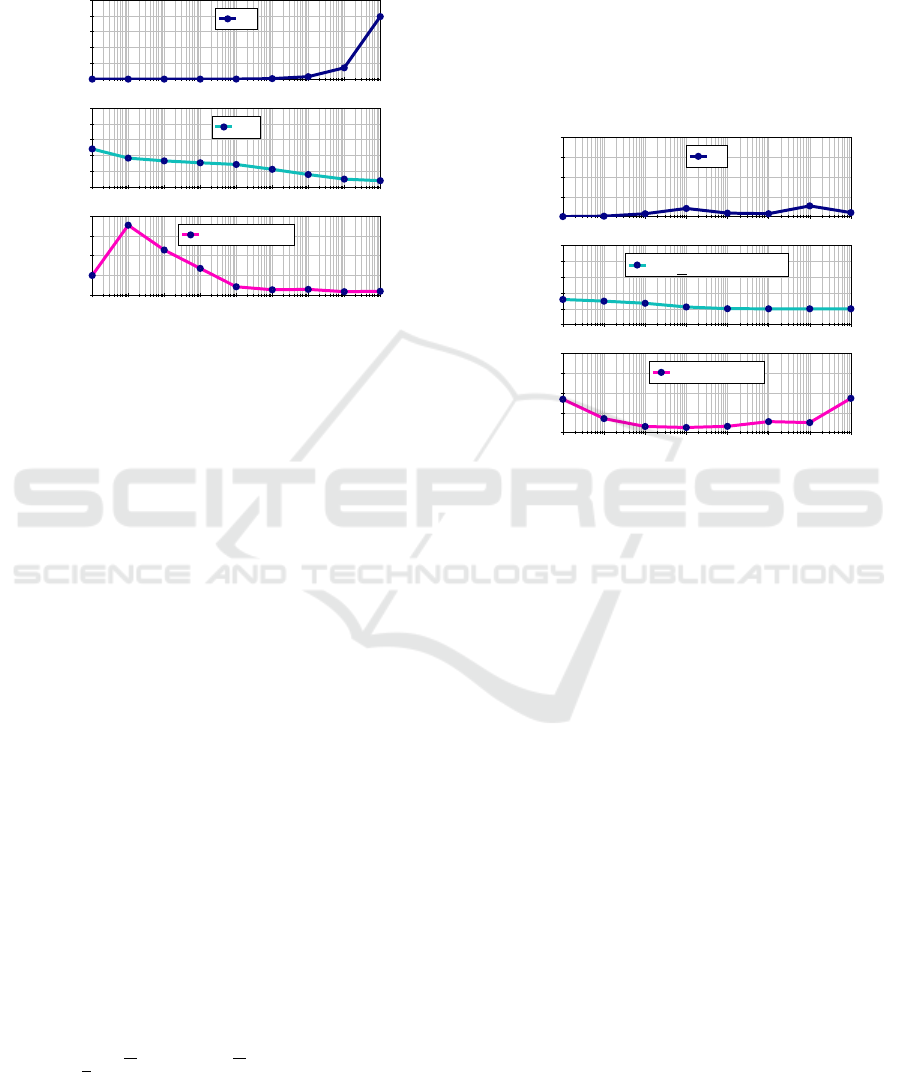
Figure 2 shows the evolution of the three space-ﬁlling

indicators as well as the loss along with the iterations.

It can be stated that all indicators detect the shrink-

age of the state trajectory and thus are validated. Note

that the absolute numerical values of the indicators are

not of interest here. The focus is only on the change

during the optimization. This is why the curves are

normalized w.r.t. their maximum values.

On closer inspection, it can be observed that the

changing curvature reveals large rates around iteration

ICINCO 2025 - 22nd International Conference on Informatics in Control, Automation and Robotics

412

0.2

0.4

0.6

0.8

Iteration

KLD CHV

Figure 2: Tracking of loss and space-ﬁlling indicators ac-

cording to the state trajectories depicted in Fig. 1.

110, indicated by the vertical line. Loosely spoken,

the optimization has already reached an acceptable ﬁt

of the process output at this point which is visible in

the loss curve. It can be concluded that space-ﬁlling

measured by those indices gets worse after the model

performance met a satisfying level. This conﬁrms that

the phenomenon of state trajectory deformation can

be seen as an overﬁtting of nonlinear state space mod-

els. This is why we recommend a regularization tech-

nique with an early-stopping effect in the next section.

4 REGULARIZED

IDENTIFICATION

Since strong state trajectory deformation is an unsat-

isfying effect, it is reasonable to design an additional

penalty for the objective that drives its data points to

a desired uniform distribution. In this section, we

present two penalty term approaches for space-ﬁlling

regularization of problem (2). Both approaches use

the ψ

described by (5) which was chosen due to im-

plementation reasons. Generally, Fig. 2 suggests that

all space-ﬁlling indicators would lead to similar re-

sults.

4.1 Space-Filling Penalty Term

As a consequence of the ψ

indicator delivering low

numerical values when data are space-ﬁlling and high

values when data are non-uniformly distributed, it

seems natural to add ψ

to the sum of the squared

output errors J in a weighted manner. The resulting

regularized problem is

min

J(θ ) + λ · ψ

(θ)

s.t. Dynamics in (2),

(7)

where λ serves as regularization strength. Exemplar-

ily, a resulting state trajectory is illustrated in Fig. 3.

Remark. The regularization technique leads to the

stabilization of the local poles due to its relocation

0.5

LM1

LM2

Figure 3: State trajectory after the optimization for λ = 10

on n

=125 grid points in three-dimensional extended in-

put/state space.

effect on data points in both LMs:

max



LM,1

)



= 0.78 < 1,

max



LM,2

)



= 0.89 < 1

Additionally, regularization enables the LMs to ex-

plain the dynamical character of the process: oscil-

lations are modeled with local complex eigenvalues,

which was not accomplished with the trajectories vis-

ible in Fig. 1. This demonstrates that the method

increases both robustness and interpretation of the

model, whereas a tradeoff regarding modeling perfor-

mance is achieved.

Next, we compare the evolution of loss J and ψ

for the regularized and unregularized problem during

the ﬁrst split optimization, see Fig. 4.

0.2

0.4

0.6

Iteration

, λ = 0 ψ

, λ = 10

J, λ = 0 J, λ = 10

Figure 4: Comparison of regularization effect on ψ

and

J. Both ψ

evolutions contain the initial space-ﬁlling at the

ﬁrst iteration with ψ

=0.23.

As already mentioned, in the unregularized case,

grows along the iterations, whereas the regular-

ized curve shows a slight decrease. This means that

the state trajectory expands during optimization. Con-

sequently, due to regularization, the loss cannot be re-

duced to J ≈ 0, because of the tradeoff between out-

put error ﬁt and space-ﬁlling of the distribution. At

termination, it reaches a level of about J ≈ 2. Further-

more, the early-stopping effect caused by the penalty

term is visible. The regularized problem is terminated

after 324 iterations whereas the baseline runs till iter-

ation 3232. This enables major savings in training

time.

Space-Filling Regularization for Robust and Interpretable Nonlinear State Space Models

413

For the choice of the hyperparameter λ , a grid

search for values between 10

−4

and 10

is carried out.

Figure 5 visualizes J, ψ

and the number of iterations.

The ﬁgure shows an increase of J for stronger reg-

100

0.2

0.4

0.6

0.8

−4

−3

−2

−1

1,000

2,000

3,000

4,000

Num. Iter.

Figure 5: Loss, space-ﬁlling and iterations after optimiza-

tion of problem (7) for various regularization strengths λ .

ularization, whereas ψ

can only be changed mod-

erately due to the dynamic relations between data

points. Since the initial state trajectory (iteration =

0, see light blue curve in Fig. 1) shows suitable space-

ﬁlling properties, it is sensible to choose λ such that

the ﬁnal state trajectory yields a similar value for ψ

As Fig. 4 shows, the initial value for ψ

= 0.23 is

obtained for a linear model in balanced realization.

This amount of space-ﬁlling can be roughly matched

at convergence after the ﬁrst split for the choice of

regularization strength of λ = 8. Independent of the

space-ﬁlling properties, λ > 1 are recommended to

realize maximum advantage w.r.t. computational de-

mand from the early-stopping (see Fig. 5, bottom di-

agram).

4.2 Desired Amount of Space-Filling

The proposed strategy requires a hyperparameter

study to ﬁnd a good value for λ. If the desired value

for space-ﬁlling is known a priori, e.g., keeping ψ

from the initial model, an alternative approach is to

penalize the deviation between the current ψ

and the

desired one (named ψ

p,Target

). By this, it represents

as a desired degree of regularization. This regularized

nonlinear problem can be stated as follows,

min

J(θ ) + λ ·



(θ) − ψ

p,Target



s.t. Dynamics in (2).

(8)

Here, a large value is chosen for the regulariza-

tion strength λ , since it simply determines the tight-

ness for matching ψ

p,Target

. For the demo process

p,Target

=0.23 is chosen, as it reﬂects the space-ﬁlling

of the initial model. Figure 6 shows the results of

the study on λ for problem (8). The loss J and the

space-ﬁlling quality ψ

are nearly independent of the

choice of λ . Therefore, it can be determined accord-

ing to the other criteria. Consequently, it is chosen as

, being a tradeoff between initial space-ﬁlling and

training time, measured by the number of iterations.

0.5

1.5

0.2

0.4

0.6

0.8

(θ) − ψ

p,Target

−1

1,000

2,000

3,000

4,000

Num. Iter.

Figure 6: Optimization results of problem (8) for various

values of λ.

5 BENCHMARK DATASET

Next, we investigate the proposed regularization strat-

egy on a well-known system identiﬁcation bench-

mark, namely the Bouc-Wen Hysteretic System. For

details on the benchmark, we refer to Schoukens and

el (2017).

For brevity, we only show the results for the De-

sired Amount of Space-Filling approach, see prob-

lem (8) in Section 4.2. For the study, the space-ﬁlling

goal is chosen as ψ

p,Target

=0.25. As for the demo pro-

cess, the regularization strength is set to λ = 10

Remark. The termination of LOLIMOT is based on

the validation error. It is terminated when no signiﬁ-

cant improvements (25 % of a normalized RMSE cor-

responding to an SNR of 40 dB) compared to the best

loss in all previous iterations can be accomplished for

three iterations. Then the simplest model within this

error range is selected.

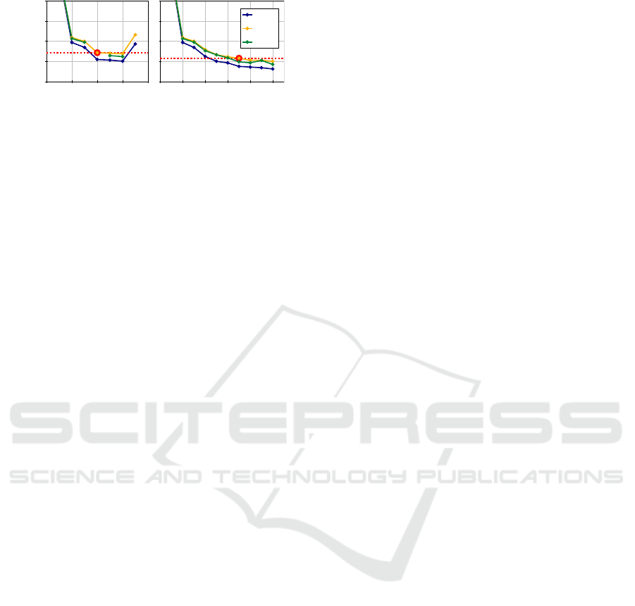
In Fig. 7, we compare the regularized and unreg-

ularized modeling cases regarding the RMSE of each

split on training, validation, and test dataset.

According to the termination criterion, the best

ICINCO 2025 - 22nd International Conference on Informatics in Control, Automation and Robotics

414

0 2 4 6 8 10

·10

−5

Split

λ = 10

0 2 4 6 8

·10

−5

Split

Error in m

λ =0

train

val

test

Figure 7: RMSE during LOLIMOT training. The best

model according to the validation error termination is

marked in red.

model for the unregularized case (λ =0) has four splits

because the validation error increases due to the sev-

enth split. This is caused by the splitting procedure

of LOLIMOT (see Sec. 2.1). The addition of a LM,

LM,x

→ n

LM,x

+ 1, requires updating the centers and

standard deviations of the Gaussians. Due to the nor-

malization, the validity functions Φ

[x]

are modiﬁed,

which in turn inﬂuences the state trajectory and thus

the output error. A poor initialization of the consec-

utive optimization of the split results and cannot be

compensated. Consequently, the training error of the

seven-split model is higher than the six-split model.

When evaluating the unregularized models on test

data, the models obtained by split numbers four and

seven show unstable behavior. In those cases, no sen-

sible RMSE can be obtained, which is why their val-

ues are omitted from the ﬁgure. Within the regular-

ized model ensemble, no instability could be detected

regarding test data. Consequently, the robustness of

LOLIMOT is improved.

Furthermore, it can be observed that regulariza-

tion allows LOLIMOT to perform seven splits for

the best model, compared to only four splits in the

unregularized case. Regularization enables the al-

gorithm to process the training dataset information

with more LMs. Evaluation on the benchmark’s test

dataset yields an RMSE of 0.981· 10

−5

m for the reg-

ularized best model, whereas the unregularized one

became unstable. In contrast to the stable splits, it

can be stated that space-ﬁlling regularization enables

better models. In comparison to other approaches,

the achieved result is among the best for this bench-

mark (Nonlinear Benchmark Working Group, 2025).

6 CONCLUSIONS

In this paper, we investigated the effect of nonlinear

optimization on the extended input/state space data

point distribution of nonlinear state space models.

Two regularization approaches for penalizing poor

space-ﬁlling quality are derived and tested, resulting

in models with more meaningful and accurate local

models. This is achieved by more local estimation

and less interpolation as well as stable local behavior.

Furthermore, higher modeling performance could be

accomplished and the number of iterations could be

reduced per optimization. Future lines of research

will focus on the stable extrapolation behavior due

to space-ﬁlling enforcement in the local model state

space network. Morevover, the applicability of space-

ﬁllling metrics with higher-dimensional settings will

be adressed.

REFERENCES

Belz, J., M

unker, T., Heinz, T. O., Kampmann, G., and

Nelles, O. (2017). Automatic modeling with local

model networks for benchmark processes. IFAC-

PapersOnLine, 50(1):470–475. 20th IFAC World

Congress.

Bemporad, A. (2024). An l-bfgs-b approach for linear and

nonlinear system identiﬁcation under ℓ

and group-

lasso regularization.

Boyd, S. and Vandenberghe, L. (2004). Convex Optimiza-

tion. Cambridge University Press.

Forgione, M. and Piga, D. (2021). Model structures and ﬁt-

ting criteria for system identiﬁcation with neural net-

works.

Garulli, A., Paoletti, S., and Vicino, A. (2012). A sur-

vey on switched and piecewise afﬁne system identiﬁ-

cation. IFAC Proceedings Volumes, 45(16):344–355.

16th IFAC Symposium on System Identiﬁcation.

Herkersdorf, M. and Nelles, O. (2025). Online and ofﬂine

space-ﬁlling input design for nonlinear system identi-

ﬁcation: A receding horizon control-based approach.

arXiv preprint arXiv:2504.02653.

Kullback, S. and Leibler, R. A. (1951). On Information and

Sufﬁciency. The Annals of Mathematical Statistics,

22(1):79 – 86.

Liu, Y., T

oth, R., and Schoukens, M. (2024). Physics-

guided state-space model augmentation using

weighted regularized neural networks.

Ljung, L. (1999). System identiﬁcation (2nd ed.): theory for

the user. Prentice Hall PTR, USA.

Ljung, L., Andersson, C., Tiels, K., and Sch

on, T. B.

(2020). Deep learning and system identiﬁcation.

IFAC-PapersOnLine, 53(2):1175–1181. 21st IFAC

World Congress.

Luenberger, D. (1967). Canonical forms for linear multi-

variable systems. Automatic Control, IEEE Transac-

tions on, AC-12:290 – 293.

McKelvey, T., Akcay, H., and Ljung, L. (1996). Subspace-

based multivariable system identiﬁcation from fre-

quency response data. IEEE Transactions on Auto-

matic Control, 41(7):960–979.

Nelles, O. (2020). Nonlinear System Identiﬁcation From

Classical Approaches to Neural Networks, Fuzzy

Space-Filling Regularization for Robust and Interpretable Nonlinear State Space Models

415

Models, and Gaussian Processes. Springer Interna-

tional Publishing; Imprint: Springer, 2020. 2nd ed.

2020., Cham.

Nonlinear Benchmark Working Group (2025). Nonlinear

benchmark models for system identiﬁcation. https:

//www.nonlinearbenchmark.org/benchmarks. Ac-

cessed: 2025-05-19.

Paduart, J., Lauwers, L., Swevers, J., Smolders, K.,

Schoukens, J., and Pintelon, R. (2010). Identiﬁcation

of nonlinear systems using polynomial nonlinear state

space models. Automatica, 46:647–656.

Pillonetto, G., Chen, T., Chiuso, A., De Nicolao, G., and

Ljung, L. (2022). Regularization for Nonlinear Sys-

tem Identiﬁcation, pages 313–342. Springer Interna-

tional Publishing, Cham.

Pintelon, R. and Schoukens, J. (2012). System Identiﬁca-

tion: A frequency Domain Approach. Wiley / IEEE

Press, 2 edition. IEEE Press, Wiley.

Rotondo, D., Puig, V., Nejjari, F., and Witczak, M.

(2015). Automated generation and comparison of

takagi-sugeno and polytopic quasi-lpv models. Fuzzy

Sets and Systems, 277.

Schoukens, M. and No

el, J. (2017). Three benchmarks ad-

dressing open challenges in nonlinear system identi-

ﬁcation. IFAC-PapersOnLine, 50(1):446–451. 20th

IFAC World Congress.

Sch

ussler, M. (2022). Machine learning with nonlinear

state space models. PhD thesis, Universit

at Siegen.

Sch

ussler, M., M

unker, T., and Nelles, O. (2019). Lo-

cal model networks for the identiﬁcation of nonlinear

state space models. In 2019 IEEE 58th Conference on

Decision and Control (CDC), pages 6437–6442.

Scott, D. (1992). Multivariate Density Estimation: The-

ory, Practice, and Visualization. A Wiley-interscience

publication. Wiley.

Smits, V. and Nelles, O. (2024). Space-ﬁlling optimized ex-

citation signals for nonlinear system identiﬁcation of

dynamic processes of a diesel engine. Control Engi-

neering Practice, 144:105821.

Suykens, J. A. K., De Moor, B. L. R., and Vandewalle, J.

(1995). Nonlinear system identiﬁcation using neural

state space models, applicable to robust control de-

sign. International Journal of Control, 62(1):129–

152.

Van Overschee, P. and De Moor, B. (1995). A unifying

theorem for three subspace system identiﬁcation al-

gorithms. Automatica, 31(12):1853–1864. Trends in

System Identiﬁcation.

Verriest, E. and Kailath, T. (1983). On generalized balanced

realizations. IEEE Transactions on Automatic Con-

trol, 28(8):833–844.

ICINCO 2025 - 22nd International Conference on Informatics in Control, Automation and Robotics

416