An Analysis to the Relationship Between Students’ GPA and

Lifestyles

Yuanhao Shen

Department of Statistic, University of Warwick, Coventry, U.K.

Keywords: Students’ GPA, Lifestyles, Relationship.

Abstract: How to have a good GPA or a great learning performance. It is a historical question, a tremendous of

investigators were trying to make a conclusion on the study efficiency depending on which situation. This

paper dives into an investigation of students from kaggle, where the data were collected from the Google

survey which was filled up by the different India university students. This paper mainly uses several

supervised machine learning algorithms to predict GPA according to different lifestyles, such as: students’

study hours per day, sleep hours per day, physical activity hours per day, extracurricular hours per day, and

stress level. In this paper, whether the regression settings or classification settings, will import the linear

regression, the polynomial regression, the logistic regression, the support vector machine (SVM), the decision

tree, the random forest, and the K-nearest neighbor (KNN) as statistical algorithms to do analysis. This article

aims to give inspiration to good GPA regarding time management.

1 INTRODUCTION

Recently, university students can join various

activities to fulfill their lives, but with limited time

every day. How to find an efficient study model is a

question in the mind. Many statisticians and scientists

were working on this region, trying to explain the

relationship between human activities and memory

improvement for example. In this case, the test of

GPA is a sufficient evidence to measure how good the

study is to students’ behavior. Supervised machine

learning, a useful and powerful tool.

To predict an object with the output of the

algorithm, which has a general name - respond; by

using different inputs, which their scientific name -

features. This paper takes the inclusion of statistical

learning models, general statistical models are linear

regression, polynomial regression, SVN, KNN, and

so forth (Biswas et al., 2021). Scientists can use these

general models for analysis by labeling the output in

the classification methods or using numerical data in

the regression setting, followed by a binary result and

its accuracy indices.

The general method involves splitting the data set

into two sections: the test set and the training set.

Additionally, the test set typically uses 20% of the

https://orcid.org/0009-0007-1968-0201

data set's observations, whereas the training set

usually uses 80%. According to ML its high

flexibility and overfitting may cause the phenomenon

that the algorithm learns about noise in the data,

rather than learning about the true distribution of the

data during training. Data splitting is crucial, it

prevents a bias made by “double dipping” with data

(Crisci et al., 2012). The discussion of the

performance index part gives the statistical analysis

of the performance of each algorithm. The reason for

using different supervised machine learning

algorithms is the data more often shows unusual

distributions, and non-linearity, the properties of

different algorithms can handle different situations

with more or less influence on the response value.

Statisticians could compare them and choose a

relatively fair algorithm as the best performance.

Machine learning has approached many science

regions and real cases in the recent years, the

consistency and the accuracy of each algorithm are

frequently mentioned (Hellström et al., 2020). The

accuracy is dominated by the test set, the same

algorithm performance can be affected slightly by the

selection observations of the training set and test set

in the raw data. This affection is irreducible and

unexpected, this impact can be ignored and cannot be

414

Shen, Y.

An Analysis to the Relationship Between Students’ GPA and Lifestyles.

DOI: 10.5220/0013698500004670

Paper published under CC license (CC BY-NC-ND 4.0)

In Proceedings of the 2nd International Conference on Data Science and Engineering (ICDSE 2025), pages 414-419

ISBN: 978-989-758-765-8

a sufficient evidence in comparing different models.

The major influence on the performance is to find the

degrees of freedom setting in each algorithm, the

higher degrees of freedom, the higher variance of the

test reducible error, and the lower bias of the estimate

observations. To verify the performance of different

statistical learning models, using error checks, for

example, the loss function can determine and find a

good parameter setting(Iniesta et al., 2016). In

general, a supervised machine learning algorithm

performance is measured on mean-squared error, or

R-square. However, measuring the performance of

the machine learning algorithm which study and

estimate binary outcomes, the accuracy, recall,

precision and F-score in the machine learning take the

significant jobs (James et al., 2023).

The main purpose of supervised machine learning

algorithms is to implement a description of the

outcome of their interests (James et al., 2023). In the

real world, data is everywhere, humans used to select

the reasonable to do research and unchanging since

times immemorial. There is an incredibly unanimous

about the fifth industrial revolution, based on fourth

industrial revolution, states that humans and machine

will work together to harmoniously contribute the

different aspects in the real world (Jain et al., 2020).

Data, as the resource to supervised machine learning,

is precious and treasured. The data widely use in

medical research, recently AlphaFold, a novel

mechine learning algorithm, based on current protein

data bank, estimate the protein structure in the high

accuracy (Jiang et al., 2020).

However, since the supervised machine learning

is data-driven. The data selection is an important and

essential step; data cleaning, noise labeling, class

imbalance, data transformation, data valuation, and

data homogeneity, all of them play a more or less

crucial role in increasing the upper prediction limit of

mechanical learning (Jumper et al., 2021).Moreover,

bias are produced from humans, similarly, machine

produce bias during the sub-tasks in the algorithm.

Scientists want to investigate the possible sources of

bias and label them to reduce the bias (Mahapatra et

al., 2022). High-quality data refers to parameters that

are sufficiently well-defined and appropriately

interpreted, as well as relevant predictors and results

that are rigorously collected. Prior to analysis, data

preprocessing requires data cleaning, data reduction

and data transformation (Noble et al., 2022).

2 METHODOLOGY

Linear regression establishes a relationship between

independent variables, such as students' study hours,

sleep hours, physical activity hours, and

extracurricular hours, and a dependent variable, GPA.

It aims to find the best-fitting line in a multi-

dimensional space by minimizing the sum of squared

residuals. When dealing with categorical features like

stress level, one-hot encoding is used to convert them

into numerical representations. Linear regression is

widely applied in predictive modeling and trend

analysis due to its simplicity and interpretability.

Polynomial regression extends linear regression

by incorporating polynomial terms of the input

features, allowing for the modeling of nonlinear

relationships. By increasing the degree of the

polynomial, the model gains more flexibility in

capturing complex data patterns. However, higher-

degree polynomials may lead to overfitting, making

regularization techniques or cross-validation essential

to balance model complexity and generalization

ability.

Logistic regression is a classification algorithm

that predicts the probability of a binary outcome by

applying the sigmoid function and mapping linear

combinations of features to probability values

between 0 and 1. The model is commonly used for

problems such as disease prediction, spam detection,

and credit risk assessment. Although logistic

regression assumes a linear decision boundary, it can

be extended to nonlinear problems using polynomial

features or kernel methods.

SVM classify data by finding the optimal

hyperplane that maximizes the margin between

different classes. It uses support vectors—data points

closest to the decision boundary—to define the

optimal separation. SVM is applicable to both linear

and nonlinear classification problems by employing

different kernel functions, such as polynomial, radial

basis function (RBF), and sigmoid kernels. Especially

in high-dimensional spaces, SVM is effective and

accurate and has been used in image recognition, text

classification, and bioinformatics.

Decision tree follows a hierarchical structure

where each node represents a decision based on

specific rules derived from the data. It splits the

dataset iteratively at each level, aiming to maximize

information gain or minimize impurity (measured by

criteria such as Gini index or entropy). Decision trees

can be easily interpret and can handle both numerical

and categorical data, but they are prone to overfitting

when the tree is too deep. Pruning techniques and

ensemble methods can help improve performance.

An Analysis to the Relationship Between Students’ GPA and Lifestyles

415

Random forest, as an ensemble learning approach,

generates multiple decision trees and combines their

outputs to enhance both accuracy and robustness. It

introduces randomness by bootstrapping samples and

selecting a subset of features for each tree, reducing

overfitting compared to individual decision trees.

Random forests are highly effective in handling

missing data, feature importance analysis, and

solving classification and regression problems.

K-nearest neighbors is a instance-based, non-

parametric learning algorithm that makes

classifications based on their proximity of new data

points to existing labeled data. It computes distances

using metrics like Euclidean, Manhattan, or

Minkowski distance and assigns the majority class

among the k-nearest neighbors. KNN is simple and

effective for pattern recognition tasks but becomes

computationally expensive with large datasets.

Optimizations such as KD-trees .and ball trees can

help speed up the process.

The formulas for accuracy, precision, recall, F1-

score followed:

Where True Positive(TP), True Negative(TN),

False Positive(FP), and False Negative(FN),

respectively.

Accuracy =

TP + TN

TP + TN + FP + FN





Precision =

TP + FN





Recall =

TP + FN





F1 − score =

2TP

2TP + FP + FN





3 EXPLORATORY DATA

ANALYSIS(EDA)

EDA as an initial stage of statistical analysis,

normally does not take any hypothesis. However, it is

a good tool to guide investigators in doing further

research.

3.1 Data Set

Table 1: This caption has one line so it is centered.

Student

Study_Hours_P

Extracurricular_Hours

Per

Sleep_Hours_P

Social_Hours_P

Physical_Activity_Hour

Per

Stress_L

evel

2 5.3 3.5 8 4.2 3

2.7

Low

3 5.1 3.9 9.2 1.2 4.6

2.6

Low

4 6.5 2.1 7.2 1.7 6.5

2.8

Moderat

5 8.1 0.6 6.5 2.2 6.6

3.5

High

2 5.3 3.5 8 4.2 3

2.7

Low

In Table 1. The student ID is a type of number

serial, it is useless and will be removed in future

analysis. Table 1 shows the Head of the dataset, and

Table 2 shows Five-point summary of the data set.

Table 2: Five-point summary of the data set.

Five

Point

Summ

ary

Study_Hours_

Per_Day

Extracurricular_Hour

s_Per_Day

Sleep_Hours_

Per_Day

Social_Hours_

Per_Day

Physical_Activity_Hou

rs_Per_Day

min 5.0 0.0 5.0 0.0 0.0 2.2

25% 6.3 1.0 6.2 1.2 2.4 2.9

50% 7.4 2.0 7.5 2.6 4.1 3.1

75% 8.7 3.0 8.8 4.1 6.1 3.3

max 10.0 4.0 10.0 6.0 13.0 4.0

ICDSE 2025 - The International Conference on Data Science and Engineering

416

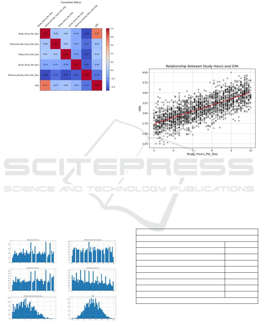
3.2 Heat Map

Figure 1: the correlation matrix.

(Picture credit: Original)

The figure 1 represent the correlation between two

numerical variables is whether positive or negative.

Each the absolute value of the correlation should in

[0,1]. The higher absolute correlation, which colors

more deeper(in cold or warm- blue or red), means that

one information can be explained by another one.

Hence produce multicollinearity to influence terribly

the correction of the regression estimations. Light

color says it has low correlation, and it is great to help

in our estimation.

In this data set, the study hours per day illustrate

its high correlation to the GPA, whereas sleeps hour

per day has the low correlation to the GPA. The

physical activities per day gives a common sense that

occupies much time in a day, hence it gives the

negative correlations to the study hours per day and

therefore GPA is negative too..

3.3 Histograms

Figure 2: Histograms of the data of the study hours per day,

extracurricular hours per day, sleep hours per day, social

hours per day, physical activity hours per day, and the GPA.

(Picture credit: Original)

In the Figure 2, the histograms of the physical

activity hours per day and the GPA are nicely

distributed on the large data. Where the histogram of

the physical activity hours per day is biased, the

histogram of GPA is relatively fair.

4 RESULTS

4.1 Linear Regression

Figure 3: Linear regression of the relationship between the

study hours per day and the GPA.

(Picture credit: Original)

The Figure 3 shows the linearity between them,

but the variance is high. The red line is the best fit

line.

characters of any form or language are allowed in

the title.

Table 3: Coefficient and R-squared, Mean Squared Error.

R-square

: 0.55

Mean Squared Erro

: 0.04

Feature Coefficient

Stud

Hours

Per

0.124126

Extracurricular

Hours

Per

-0.038298

Slee

Hours

Per

-0.030098

Social_Hours_Per_Da

-0.027520

Physical_Activity_Hours_Per_Day -0.028211

Stress

h 0.006212

Stress

Low 0.010818

Stress

Moderate -0.017030

Intercept: 2.6869435637219166

In the table 3, the Study Hours Per Day perform

as a good estimator, that the coefficient is large,

where the others are not.

An Analysis to the Relationship Between Students’ GPA and Lifestyles

417

𝑅



= 1 −

𝑈𝑛𝑒𝑥𝑝𝑎𝑖𝑛𝑒𝑑 𝑉𝑎𝑟𝑖𝑎𝑡𝑖𝑜𝑛

𝑇𝑜𝑡𝑎𝑙 𝑉𝑎𝑟𝑖𝑎𝑡𝑖𝑜𝑛





The coefficient of determination R is 0.55, that

means there are 45% of the estimation from hidden

variables, only 55% of the features are collected in the

data set. Hence, more variance needed to produce a

better estimation.

The mean squared error MSE is 0.04, n is 2000.

MSE =





real Y − estimate Y













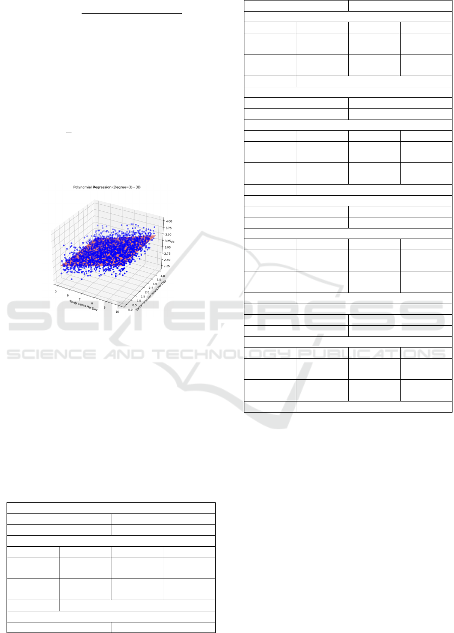
4.2 Polynomial Regression(3-D)

Figure 4: A 3-D polynomial plot.

(Picture credit: Original)

The figure 4 exibit an estimation, given that

polynomial degree = 3. Estimate the response of GPA

with features of Study Hours Per Day and

Extracurricular Hours Per Day .

4.3 Classification Settings

As predict binary output, this design divide and label

the students’ GPA into the above half(GPA greater

than 3.1) and the below half(GPA equal and less than

3.1), where the 3.1 is the median of the GPA.

Table 4: Classification settings and classification reports.

Model: Lo

istic Re

ression

Accurac

: 0.775000 Precision: 0.775000

Recall: 0.775000 F1 Score: 0.775000

Classification Report:

recision recall f1-score

Above

Half

0.77 0.77 0.77

Below

Half

0.78 0.78 0.78

accurac

0.78

Model: SVM

Accuracy: 0.762500 Precision: 0.763460

Recall: 0.762500 F1 Score: 0.762171

Classification Report:

recision recall f1-score

Above

Half

0.78 0.73 0.75

Below

Half

0.75 0.80 0.77

accurac

0.76

Model: Decision Tree

Accuracy: 0.647500 Precision: 0.647521

Recall: 0.647500 F1 Score: 0.647507

Classification Re

ort:

recision recall f1-score

Above

Half

0.64 0.64 0.64

Below

Half

0.65 0.65 0.65

accurac

0.65

Model: Random Forest

Accurac

: 0.737500 Precision: 0.737593

Recall: 0.737500 F1 Score: 0.737505

Classification Report:

recision recall f1-score

Above

Half

0.74 0.73 0.74

Below

Half

0.74 0.73 0.74

accurac

0.64

Model: KNN

Accuracy: 0.762500 Precision: 0.765114

Recall: 0.762500 F1 Score: 0.762076

Classification Re

ort:

recision recall f1-score

Above

Half

0.74 0.81 0.77

Below

Half

0.79 0.72 0.75

accurac

0.76

In the table 4, each of the algorithms perform very

close, there is no a very prominent algorithm. The

accuracy of each machine learning algorithm is

around 0.75. Based all outputs, the logistic regression

algorithm has a slight advantage over other. Which

takes the 0.775 on both accuracy, recall, precision, F1

Score, achieve high accuracy stated.

SVM, the second ML model, has the accuracy

0.7625, recall 0.7625, precision 0.76346, F1-score

around 0.762171. KNN shows its good performance,

which accuracy is 0.7625, recall is 0.7625, precision

is 0.765114, F1-score is around 0.762076. Random

forest and decision tree are not performed good to

estimate in this situation, the former one accuracy is

0.7375, recall is 0.7375, precision is around

0.737593, and F1-score is 0.737505; where the later

one accuracy is 0.6475, recall is 0.6475, recall is

around 0.647521, F1-score is around 0.647507.

ICDSE 2025 - The International Conference on Data Science and Engineering

418

5 CONCLUSIONS

Algorithms predict responses in these patterns but

cannot achieve high accuracy. This is not sufficient

proof or confidence to claim that the models have

significantly improved, as the accuracy on the test

result is not consistent across different tests. One

problem is that the sampling process has not a strict

rule, therefore both random errors and bias effect the

result. As the result shows that the sleeping hours per

day has very low correlation to the GPA, where

sleeping is important to improve memory, and

directly effect on the GPA. But not surprisingly, the

study hours per day is a good predictor, and at least 8

hours study per day is needed if students want to have

a good GPA. Another problem is the data set is not

large, only 2000 observations which can see the

supervised machine learning can not perform well if

there is not a such sufficient data to support, and

investigator can spend more time on correcting the

feature and response labels to reach high accuracy.

This result shows that the expect study time everyday

that study needed to reach a high GPA.

REFERENCES

Biswas, A., Saran, I., & Wilson, F. P. (2021). Introduction

to supervised machine learning. Kidney360, 2(5), 878–

880.

Crisci, C., Ghattas, B., & Perera, G. (2012). A review of

supervised machine learning algorithms and their

applications to ecological data.

Hellström, T., Dignum, V., & Bensch, S. (2020). Bias in

machine learning—What is it good for?

Iniesta, R., Stahl, D., & McGuffin, P. (2016). Machine

learning, statistical learning and the future of biological

research in psychiatry. Psychological Medicine, 46(12),

2455–2465.

James, G., Witten, D., Hastie, T., Tibshirani, R., & Taylor,

J. (2023). An introduction to statistical learning with

applications in Python (Vol. 1). Springer.

Jain, A., Patel, H., Nagalapatti, L., Gupta, N., Mehta, S.,

Guttula, S., Mujumdar, S., Afzal, S., Mittal, R. S., &

Munigala, V. (2020). Overview and importance of data

quality for machine learning tasks. In Proceedings of

the 26th ACM SIGKDD International Conference on

Knowledge Discovery & Data Mining (pp. 3561–

3562). Association for Computing Machinery.

Jiang, T., Gradus, J. L., & Rosellini, A. J. (2020).

Supervised machine learning: A brief primer. Behavior

Therapy, 51(5), 675–687.

Jumper, J., Evans, R., Pritzel, A., et al. (2021). Highly

accurate protein structure prediction with AlphaFold.

Nature, 596, 583–589.

Mahapatra, R. P., et al. (Eds.). (2022). Proceedings of

International Conference on Recent Trends in

Computing. Lecture Notes in Networks and Systems

(Vol. 600). Springer.

Noble, S. M., Mende, M., Grewal, D., & Parasuraman, A.

(2022). The fifth industrial revolution: How

harmonious human–machine collaboration is triggering

a retail and service [r]evolution. Journal of Retailing,

98(2), 199–208.

Smith, J., 1998. The book, The publishing company.

London, 2nd edition.

An Analysis to the Relationship Between Students’ GPA and Lifestyles

419